Abstract
Shock signal features must be extracted for use in pattern recognition or fault diagnosis. In this work, we proposed a method for the feature extraction of shock signals, which are vibration signals that change faster and have larger amplitude ranges than general signals. First, we proposed the concepts of amplitude density for monotonic functions and piecewise monotonic functions. On the basis of these concepts, we then proposed the concept of the upper limit of density integral (ULDI), which was adopted to obtain signal features. Then, we introduced two types of serious fault cracks to the latch sheet of an automatic gun mechanism that is used on warships. Next, we applied the proposed method to extract the features of shock signals from data acquired when the automatic gun mechanism fired with normal and two fault patterns. Finally, we verified the effectiveness of our proposed method by applying the features that it extracted to a support vector machine (SVM). Our proposed method provided good results and was superior to the traditional statistics-based feature extraction method when applied to a SVM for classification. In addition, the former method demonstrated better generalisation than the latter. Thus, our method is an efficient approach for extracting shock signal features in pattern recognition and fault diagnosis.
Highlights
- We proposed the concept of upper limit of density integral to obtain signal features.
- The proposed method was applied to extract the features about an automatic gun mechanism.
- The proposed method was superior to the traditional statistics-based feature extraction method.
1. Introduction
Shock signal features must be extracted for utilisation in pattern recognition or fault diagnosis. Methods for the extraction of shock signal features can be classified into two major categories in accordance with the space wherein the signal exists. Methods in the first category involve the direct extraction of the features of an original signal in the time domain; commonly used methods in this category include mathematical statistics, information entropy [1-4]. Methods in the second category involve signal decomposition or transformation followed by feature extraction. Examples of commonly used signal decomposition methods in this category include various filter methods and empirical mode decomposition [5-8]. Commonly applied signal transformation methods include Fourier transform, wavelet transform [9, 10] and Hilbert transform. In fault diagnosis, we first use these methods to obtain the original signal features. Then, we use other methods, such as genetic algorithm [11-14], principal component analysis [15, 16] and kernel principal component analysis [17, 18] to perform necessary selections and transformations to obtain the appropriate features.
Many scholars have improved the classical algorithms for signal feature extraction. Yang and Nataliani [19] presented a novel method for improving fuzzy clustering algorithms that can automatically compute individual feature weight and simultaneously reduce irrelevant feature components. They first considered the objective function of fuzzy c-means with feature-weighted entropy, constructed a learning schema for parameters and then reduced irrelevant feature components. Saif et al. [20] proposed the application of the nonlinear complete ensemble empirical mode decomposition method with adaptive white noise to decompose signals into intrinsic mode functions (IMFs). Deng et al. [21] revealed the inherent characteristics of vibration signals by calculating the fuzzy information entropy values of IMFs and considering them as feature vectors. They then proposed an improved particle swarm optimisation (PSO) algorithm by using the diversity mutation, neighbourhood mutation, learning factor and inertia weight strategies for the basic PSO. Finally, they used the improved PSO algorithm to optimise the parameters of least squares support vector machines (LS-SVM) for the construction of an optimal LS-SVM classifier. Zhao et al. [22] proposed an enhanced empirical wavelet transform (MSCEWT) based on the maximum-minimum length curve method. The proposed MSCEWT can obtain fewer IMFs than empirical mode decomposition and ensemble empirical mode decomposition.
Original features affect the accuracy of pattern recognition and fault diagnosis, and additional signal properties can be fully reflected by increasing the number of features. The features that can represent the main properties of signals with different properties may vary. Therefore, developing a new method for signal feature extraction is crucial. In this work, we proposed a method for extracting shock signal features. We first proposed the concept of the amplitude density of a signal. Then, we proposed the concept of the ULDI, which is adopted for signal feature extraction. Finally, we analysed the features of shock signals for an automatic gun mechanism to verify the effectiveness of our proposed method.
2. Amplitude density and density integral
2.1. Amplitude density for monotonic functions
Assume that a signal is defined in the interval and satisfies 0, where , . The functional image of is presented in Fig. 1.
Fig. 1Functional image of ft
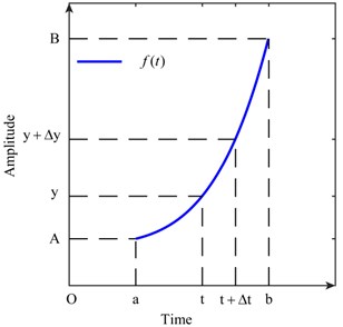
Then, Eq. (1) is established by considering points and in :
We define a function that satisfies Eq. (2):
Both ends of Eq. (2) are divided by . The limit is taken as Eq. (3). Then, Eq. (3) becomes equal to Eq. (4):
is defined as the amplitude density function of in the interval . reflects the probability of that takes in the interval . 0 exists, and Eq. (5) is true. The opposite number of the right end in Eq. (4) when 0 is taken. Eq. (6) is thus established:
2.2. Amplitude density for piecewise monotonic functions
Assume that a signal that is defined in the interval can be divided intoamounts of monotonic intervals and the derived function , exists where:
The functional image of is illustrated in Fig. 2. The piecewise function in every monotonic interval is assumed to be expressed as , 1, 2, ..., .
Fig. 2Function ft that is defined in finite monotonic intervals
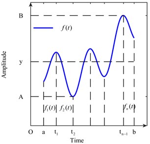
Considering the amplitude density of , the piecewise function , and is assumed to take the value. On the basis of our analysis in section 2.1, we show that the amplitude density , where , should be established as (7):
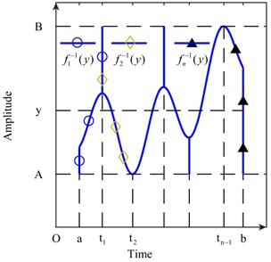
The interval of the definition of the piecewise inverse function , 1, 2, ..., , is extended. The result of the extension is plotted in Fig. 3. For every extreme point or end point in , the minimum points are extended to , and the maximum points are extended to . The piecewise inverse function that has been extended is still expressed as , , 1, 2, …, to facilitate expression in this paper. Therefore, Eq. (7) is equal to Eq. (8). We can still consider as the amplitude density function of :
Fig. 3Extended piecewise inverse functions
2.3. ULDI
Both ends of Eq. (8) are subjected twice to the definite integral operation in the interval and , , of which the result is Eq. (9):
let:
then, Eq. (9) is equal to Eq. (10):
We can ignore the influence of inverse functions without differential coefficients at the extreme points or end points of when we calculate Eq. (10). Therefore, the value of , and 1, 2, ..., at the local area of these points is readjusted to ensure that exists, whereas the value of remains unchanged. We can handle this operation in this manner because the value of the integral is unchanged by standard integration and changing the integrand on a set of zero measure does not change the value of the integral (measure theory).
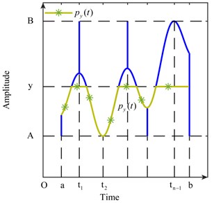
The area of the shaded regions in Fig. 4 is regarded as . Eq. (11) is true. Furthermore, we regard the curve in Fig. 5 as , which is formed by and the constant:
is easily obtained whenis determined. On the other hand, can be expressed as Eq. (12):
We can obtain Eq. (13) by combining Eqs. (10), (11) and (12). Then, Eqs. (14) and (15) are true:
, and are uniquely determined by each other when is determined. We designate as the ULDI of a signal. The data obtained in engineering applications are discrete. The error of the first-order differential operation is low in the calculation of the differential operation of Eq. (14). When solving the second-order differential operation in Eq. (15), the local of the first-order differential section steps into a jump. The second-order differential is therefore not consistent with the actual value if the differential region is small. On the other hand, if the differential region is large, the accuracy of the calculation will decrease. Signal features will be extracted by utilising Eq. (14) to avoid this problem.
Fig. 4Area Sy of the shaded regions
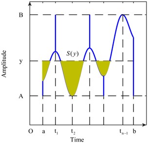
Fig. 5Curve of Pyt
3. Features of shock signals
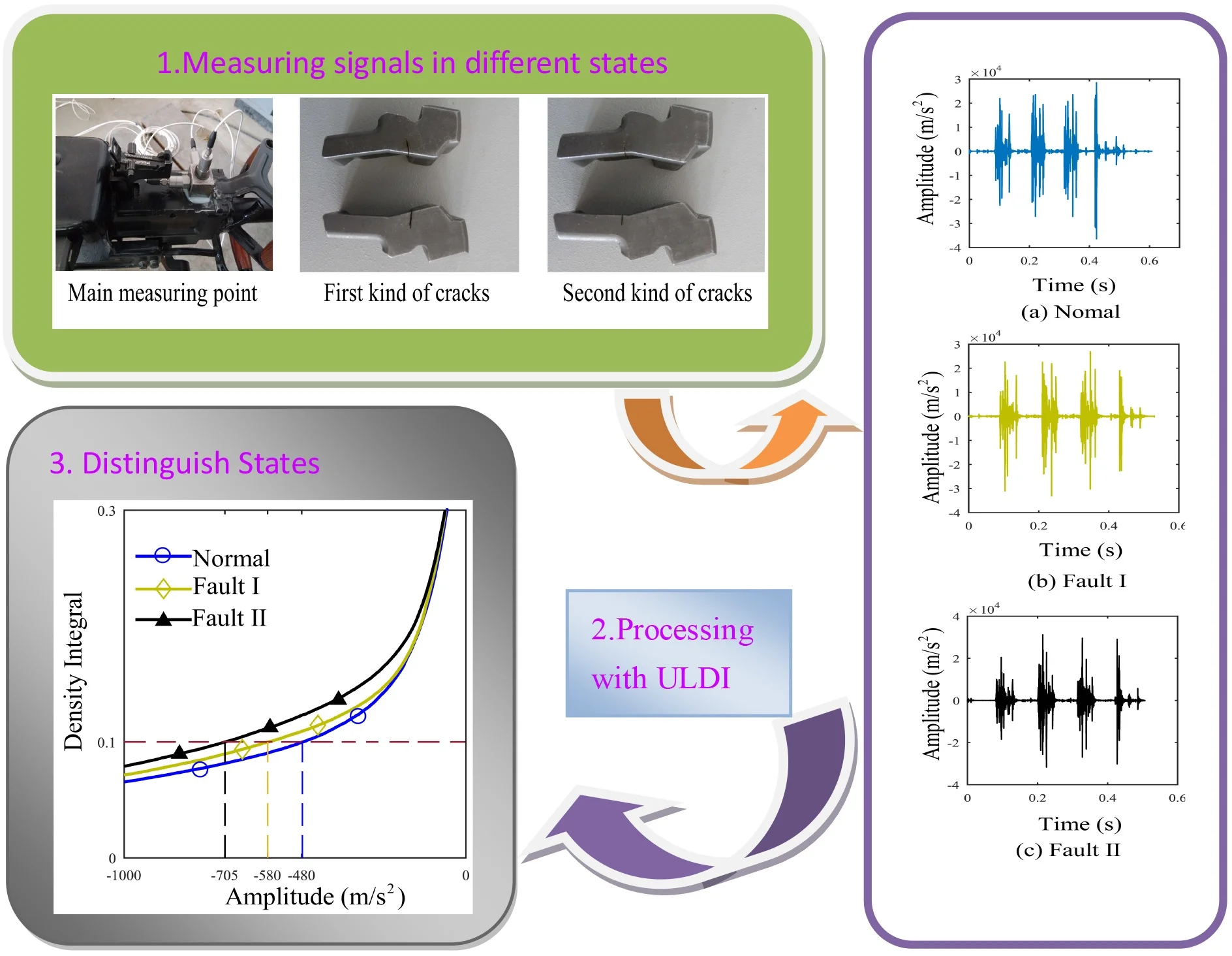
As discussed in this section, we introduced two types of serious fault cracks to the latch sheet of an automatic gun mechanism that is used on warships. Then, we applied the proposed method to extract the features of shock signals from data acquired when the automatic gun mechanism fired with normal and two fault patterns. The firing frequency of the automatic gun mechanism is 10 Hz. The main parameters of the sensors that we used in this work are shown in Table 1.
Table 1Sensor parameters
Performance | Value |
Sensitivity | 1.0 mV/g (±15%) |
Measurement range | ± 5,000 g pk |
Frequency range | 0.4 Hz to 7,500 Hz (±10 %) |
Electrical filter cutoff frequency | ≥7.5 kHz (−10 %) |
Resonant frequency | ≥50 kHz |
Broadband resolution | 0.02 g rms (1kHz to 10 kHz) |
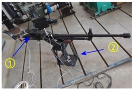
We set the sampling frequency as the maximum sampling frequency (204.8 kHz) of the signal collector to obtain additional details in the time domain and the sampling time as 5 s. The environmental parameters of the experiment are shown in Fig. 6. The main measuring point and the two types of serious fault cracks are illustrated in Fig. 7.
Fig. 6Environment of the experiment
a) The position prone to noise
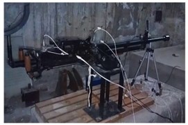
b) The place for experiment
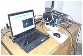
c) Signal collector
Fig. 7Main measuring point and two types of serious fault cracks

a) The main measuring point
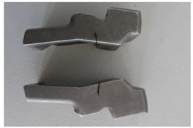
b) The first kind of cracks
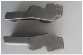
c) The second kind of cracks
3.1. ULDI of shock signals
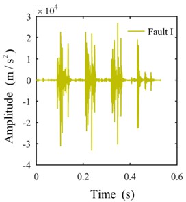
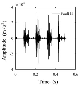
Only the actual effective time period of the original signal is intercepted for analysis to avoid the interference of invalid signals with effective signals. The shock signals in the time domain are plotted in Fig. 8. The ULDIs of each signal are shown in Fig. 9. The area [–1000, 0]×[0, 0.3] of Fig. 9 is presented in Fig. 10 to properly illustrate the ULDI of each signal. From Fig. 10, we can conclude that under the same density integral, the amplitudes that correspond to different working modes are different.
Fig. 8Signals in the time domain
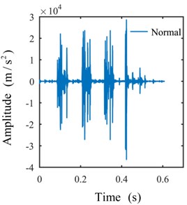
a)
b)
c)
3.2. Signal features
For a continuous shock signal , the ULDI is a strictly monotonically increasing function of . Therefore, for a determined value of , we can obtain the amplitude that corresponds to through bisection, which is a method that is commonly used to identify zero points. The amplitudethat corresponds to a determined value of can be denoted as , , , , where means the index of signals generated by different patterns, means the index of signals generated by same pattern and means the index of amplitudes that correspond a signal.
Fig. 9Density integrals of signals
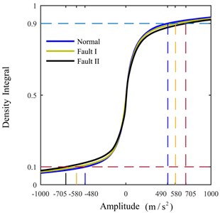
Fig. 10Area [–1000,0]×[0,0.3] of Fig. 9
![Area [–1000,0]×[0,0.3] of Fig. 9](https://static-01.extrica.com/articles/20207/20207-img16.jpg)
Three signals that correspond to the different firing pattern with respect to the different values of are shown in Table 2, which means , , and . Therefore, we can consider , 8, as the feature of a signal. From Table 2, we can infer that the difference between the different work patterns first decreases and then increases as the density integral increases. This behaviour reflects the similarities and differences between each firing pattern.
Table 2Signal features
Density integral | 0.1 | 0.2 | 0.3 | 0.4 | 0.5 | 0.6 | 0.7 | 0.8 | |
Amplitude (m/s2) | Normal | −478.13 | −138.11 | −62.67 | −23.41 | 1.24 | 24.53 | 64.67 | 151.75 |
Fault I | −579.77 | −149.66 | −65.09 | −25.29 | −0.02 | 25.03 | 70.32 | 161.02 | |
Fault II | −704.80 | −185.57 | −65.76 | −17.61 | 1.37 | 24.90 | 77.01 | 180.88 | |
3.3. Applying extracted features to a SVM
We further verified the effect of our proposed method and selected the data from one sensor for verification (there are 8 sensors in the actual test of sampling signals). We sampled 14 effective groups of data that correspond to each work pattern for application into an SVM, and limited by the service life of the automatic gun mechanism. Only small samples can be sampled. The steps of feature extraction and verification are as follows.
Step 1: on the base of original signals, intercept the signal segment when the latch sheet is working.
Step 2: the instantaneous frequency function of IMF2 is obtained by EMD decomposition of the signal that is intercepted.
Step 3: on the base of instantaneous frequency function of IMF2, we extracted the features that are similar to the features presented in Section 3.2.
Above what we analysed, there are 42 samples (features) for classification. At the process of training and testing SVM, we chose to leave one out cross validation. The results of the training are presented in Table 3, and the results of testing are provided in Table 4 [23-25].
The dimensionality of the features used for the SVM is 11, and 11. We selected the radial basis function (RBF) as the kernel of the SVM. The kernel is expressed as:
0, of which is the width and was selected as 5.
We validated the effectiveness of the proposed method by comparing its performance with that of a statistics-based method. We selected the same sample data and SVM parameters for classification. In general, we can represent the instantaneous frequency data that correspond to a shock signal as . Table 5 shows the representation of each component of the feature extracted from signals on the basis of mathematical statistics. We can regard this feature as . The dimensionality of the features is 8. Training results are shown in Table 6, and testing results are shown in Table 7.
From Tables 3 and 4, we can infer that the SVM conflates features that correspond to normal patterns with those that correspond to fault I patterns. Although the classification results are acceptable, accuracy must be improved by combining other types of features. As inferred from Tables 4 and 7, the classification performance of the proposed method is superior to that of the traditional method that constructs features on the basis of mathematical statistics. Tables 3, 4, 6 and 7 show that the generalisation of the former method is better than that of the latter method.
Table 3Results of SVM training
Training | Normal | Fault I | Fault II |
Normal | 13 | 0 | 0 |
Fault I | 1 | 14 | 1 |
Fault II | 0 | 0 | 13 |
Accuracy (%) | 92.85 | 100 | 92.85 |
Table 4Results of SVM testing
Test | Normal | Fault I | Fault II |
Normal | 12 | 1 | 0 |
Fault I | 2 | 12 | 1 |
Fault II | 0 | 1 | 13 |
Accuracy (%) | 85.71 | 85.71 | 92.85 |
Table 5Feature representation
Feature components | Representation | Feature components | Representation |
Absolute mean | Wave form | ||
Peak value | Peak index | ||
Mean square | Impulse index | ||
Root square | Skewness |
Table 6Training results for the features constructed on the basis of mathematical statistics
Training | Normal | Fault I | Fault II |
Normal | 12 | 0 | 0 |
Fault I | 2 | 13 | 1 |
Fault II | 0 | 1 | 13 |
Accuracy (%) | 85.71 | 92.85 | 92.85 |
Table 7Testing results for features constructed on the basis of mathematical statistics
Test | Normal | Fault I | Fault II |
Normal | 12 | 1 | 1 |
Fault I | 2 | 11 | 0 |
Fault II | 0 | 2 | 13 |
Accuracy (%) | 85.71 | 78.57 | 92.85 |
4. Conclusions
We proposed a method for extracting shock signal features. The proposed method has low computational cost. Given this characteristic, our proposed method can be used as a simple and efficient tool for the extraction of shock signal features for pattern recognition or fault diagnosis. Using the features extracted by our proposed method in pattern recognition yielded good results. Nevertheless, other types of features must be combined to improve identification accuracy.
The shock signals used in this work are deterministic signals, which are repeatable. Thus, the proposed method can reliably and robustly differentiate different signal types. However, this method is not necessarily applicable to signals that are corrupted and is sensitive to the time domain partition. Signals in the time domain must be first partitioned prior to the application of the proposed method to avoid these problems.
References
-
Zhao M. Y., Xu G. Feature extraction of power transformer vibration signals based on empirical wavelet transform and multiscale entropy. IET Science, Measurement and Technology, Vol. 12, Issue 1, 2018, p. 63-71.
-
Kumar M., Pachori R. B., Acharya U. R. An efficient automated technique for CAD diagnosis using flexible analytic wavelet transform and entropy features extracted from HRV signals. Expert Systems with Applications, Vol. 63, Issue 30, 2016, p. 165-172.
-
Das A. B., Bhuiyan M. I. H. Discrimination and classification of focal and non-focal EEG signals using entropy-based features in the EMD-DWT domain. Biomedical Signal Processing and Control, Vol. 29, 2016, p. 11-21.
-
Sun J., Li H. R., Xu B. H. Degradation feature extraction of the hydraulic pump based on high-frequency harmonic local characteristic-scale decomposition sub-signal separation and discrete cosine transform high-order singular entropy. Advances in Mechanical Engineering, Vol. 11, Issue 1, 2009, p. 17-26.
-
Huang E., Shen Z., Long S. R., et al. The empirical mode decomposition and the Hilbert spectrum for nonlinear and non-stationary time series analysis. Proceedings Mathematical Physical and Engineering Sciences, Vol. 454, Issue 1974, 1998, p. 903-995.
-
Veltcheva A. D., Guedes Soares C. Identification of the components of wave spectra by the Hilbert Huang transform method. Applied Ocean Research, Vol. 26, Issues 1-2, 2004, p. 1-12.
-
Alvanitopoulos P. F., Papavasileiou M., Andreadis I., Elenas A. Identification of the components of wave spectra by the Hilbert Huang transform method. IEEE Transactions on Instrumentation and Measurement, Vol. 61, Issue 2, 2012, p. 326-337.
-
Roy A., Wen C. H., Doherty J. F. Signal feature extraction from microbarograph observations using the Hilbert-Huang transform. IEEE Transactions on Geoscience and Remote Sensing, Vol. 46, Issue 5, 2008, p. 1442-1447.
-
Ghasemzadeh A., Demirel H. 3D discrete wavelet transform-based feature extraction for hyperspectral face recognition. IET Biometrics, Vol. 7, Issue 1,2018, p. 49-55.
-
Wang T., Li L., Huang Y. A., et al. Prediction of protein-protein interactions from amino acid sequences based on continuous and discrete wavelet transform features. Molecules, Vol. 23, Issue 4, 2018, p. E823.
-
Gauthama Raman M. R., Somu N., Kirthivasan K., Liscano R., Shankar Sriram V. S. An efficient intrusion detection system based on hypergraph-genetic algorithm for parameter optimization and feature selection in support vector machine. Knowledge-Based Systems, Vol. 134, Issue 15, 2017, p. 1-12.
-
Ma B. T., Xia Y. A tribe competition-based genetic algorithm for feature selection in pattern classification. Applied Soft Computing, Vol. 58, 2017, p. 328-338.
-
Li H. Q., Yuan D. Y., Ma X. D., Cui D. Y., Cao L. Genetic algorithm for the optimization of features and neural networks in ECG signals classification. Scientific Reports, Vol. 7, 2017, p. 41011.
-
Lei L., Yan J. H., de Silva C. W. Feature selection for ECG signal processing using improved genetic algorithm and empirical mode decomposition. Measurement, Vol. 94, 2016, p. 374-381.
-
Shah S. M. S., Batool S., Khan I., et al. Feature extraction through parallel probabilistic principal component analysis for heart disease diagnosis. Physica A: Statistical Mechanics and its Applications, Vol. 482, 2017, p. 796-807.
-
Luss R., D’Aspremont A. Clustering and feature selection using sparse principal component analysis. Optimization and Engineering, Vol. 11, Issue 1, 2010, p. 145-157.
-
Sahu A., Apley D. W., Runger G. C. Feature selection for noisy variation patterns using kernel principal component analysis. Knowledge-Based Systems, Vol. 72, 2014, p. 37-47.
-
Schölkopf B., Smola A., Müller K. R. Nonlinear component analysis as a kernel eigenvalue problem. Neural Computation, Vol. 10, Issue 5, 1998, p. 1299-1319.
-
Yang M. S., Nataliani Y. A Feature-reduction fuzzy clustering algorithm based on feature-weighted entropy. IEEE Transactions on Fuzzy Systems, Vol. 26, Issue 2, 2018, p. 817-835.
-
Saif N., Amalin P., Anita A. Entropy-based feature extraction and classification of vibroarthographic signal using complete ensemble empirical mode decomposition with adaptive noise. IET Science, Measurement and Technology, Vol. 12, Issue 3, 2018, p. 350-359.
-
Deng W., Yao R., Zhao H., et al. A novel intelligent diagnosis method using optimal LS-SVM with improved PSO algorithm. Soft Computing, 2017, https://doi.org/10.1007/s00500-017-2940-9.
-
Zhao H., Zuo S., Hou M., et al. A novel adaptive signal processing method based on enhanced empirical wavelet transform technology. Sensors, Vol. 18, Issue 10, 2018, p. 3323.
-
Cristianini N., Shawe-Taylor J. An Introduction to Support Vector Machines and Other Kernel-based Learning Methods. Cambridge University, London, 2000.
-
Theodoridis S., Koutroumbas K. Pattern Recognition. Linear Classifiers. 4th Edition, Elsevier, Burlington, MA, USA, 2009.
-
Russell S. J., Norvig P. Artificial Intelligence: a Modern Approach. Learning from Examples. 3rd Edition, Pearson Education, Upper Saddle River, NJ, USA, 2010.
About this article

The authors gratefully acknowledge the support from the National Natural Science Foundation of China (Grants 51675491 and 51175480).
