Abstract
In the fault diagnosis of the shaft orbit of rotating machinery, there are few prejudgments about the severity of the faults, which is very important for fault repair. Therefore, a fine-grained recognition method is proposed to detect different severity faults by shaft orbit. Since different shaft orbits represent different type and different severity of faults, the convolutional neural network (CNN) is applied for identifying the shaft orbits to recognize the type and severity of the fault. The recognition rate of proposed fine-grained fault identification method is 97.96 % on the simulated shaft orbit database, and it takes only 0.31 milliseconds for the recognition of single sample. Experimental result indicated that the classification performance of the proposed method are better than the traditional machine learning models. Moreover, the method is applied for the identification of the measured shaft orbits of rotor with different degree of imbalance faults, and the testing accuracy of the experiments in measured shaft orbits is 97.14 %, which has verified the effectiveness of the proposed fine-grained fault recognition method.
Highlights
- A fine-grained recognition method is proposed to detect different severity faults by shaft orbit.
- CNN is applied for identifying the shaft orbits to recognize the type and severity of the fault.
- The proposed method achieve good recognition and has a guiding role in the actual fault diagnosis of rotating machinery.
1. Introduction
With the continual development of industry, the structure of rotating machinery is getting more and more complicated. Due to the severe working environment, the rotating machinery is inevitably subject to various faults, which will lead to serious accidents and casualties [1]. Therefore, condition monitoring and fault diagnosis for these key rotating machinery are important for increasing production efficiency, decreasing maintenance charges, and extending service life of the equipment [2, 3].
Faults of rotating machinery are usually characterized as shaft abnormal vibrations [4]. Monitoring and diagnosis of shaft vibration signals are still the main means for the maintenance of rotating machinery, and shaft orbit synthesized by these vibration signals is an important tools for fault diagnosis [2]. Shaft orbit contains abundant information about the shaft working state, and the shaft orbit shape could accurately reflect the running state and fault condition of rotating machinery, such as outer “8” and banana shapes corresponding to shaft misalignment, ellipse corresponding to shaft unbalance [5].
However, there are no clear boundaries between different faults. For example, shaft orbit may change from ellipse to outer “8” shape when the severity of the shaft misalignment increases [6]. Therefore, it is not good enough to identify the graphic merely, and it is necessary to identify the severity of faults reflected by shaft orbits. The ellipse orbit shape with different length-width ratios corresponds to the different fault information, and the difference in the size of the two rings of the outer “8” shape also represents different severity of shaft misalignment [6]. Therefore, there is an urgent need for a method to finely recognize the shape and degree of the shaft orbits.
Traditional identification methods of shaft orbits include three steps: preprocessing, feature extraction, and classification. However, it is always a difficult problem to choose the appropriate feature descriptors and the corresponding classifier. The common feature descriptors used in the identification of shaft orbit are Fourier descriptors (FD) [7], chain code [8], Walsh descriptor (WD) [9], Hu invariant moment [10], histogram of oriented gradients (HOG) [11], comprehensive geometric characteristic (CGC) [2] and accurate Fourier height functions (AFHF) [12]. The commonly used classifiers are BP neural network [10] and support vector machine (SVM) [12]. These traditional pattern recognition methods can only distinguish different kinds of shaft orbits. The features extracted by these methods are not suitable for the identification of fine-grained shaft orbits.
The classification performance of traditional methods depends on the feature descriptors to a large extend. Unlike the traditional methods, convolutional neural network (CNN) can automatically extracts features from data. It has higher recognition accuracy and stronger anti-interference ability. At present, CNN has been successfully applied in fault diagnose of rotating machinery. Feature maps reconstructed by the raw vibration signals are usually used as the input of CNN, the reconstruction methods mainly include time-frequency analysis [13-17], time series permutation [18] and division of vibration signal map [19-21]. However, those feature maps have more complex physical meanings than shaft orbits, which can directly reflect the change of shaft position and the severity of the fault, and the CNN was rarely used in shaft orbit recognition. Therefore, a fine-grained fault recognition method for shaft orbit of rotary machine based on CNN is proposed in this paper. First, the theory of fine-grained shaft orbit is proposed to divide different shaft orbits into several subclasses which reflect the different severity of the fault. Then, the appropriate network structure of CNN is designed to identify the fine-grained shaft orbits.
The structure of this paper is arranged as following: the corresponding relationship between the severity of faults and fine-grained shaft orbits is analyzed in Section 2.1. The classification method of fine-grained shaft orbits based on improved LeNet-5 is described in Section 2.2. The experiments about the optimal structure of proposed CNN are presented in Section 3.1. The experiment on the identification of fine-grained shaft orbits is introduced in Section 3.2 and 3.3. Finally, conclusions of this paper are summarized in Section 4.
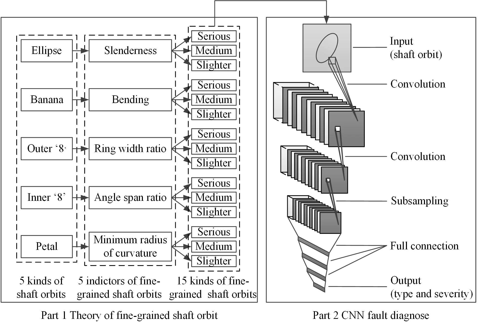
Fig. 1Flow chart of proposed identification method of fine-grained shaft orbits based on improved LeNet-5
2. Identification method of fine-grained shaft orbits based on improved LeNet-5
As discussed above, the shape of shaft orbits can reflect the type and the severity of faults. A new theory of fine-grained shaft orbits is proposed in this section to divide different shaft orbits into several subclasses that can reflect the severity of the fault. In addition, a CNN based on improved LeNet-5 are introduced to identify fine-grained shaft orbits. Fig. 1 illustrates the procedure of the proposed method, which consists of two parts: the theory of fine-grained shaft orbits and the optimized CNN classification method. Details of each part of the proposed method are described below.
2.1. Modeling of fine-grained shaft orbit with different severity of faults
2.1.1. Theory of fine-grained shaft orbit
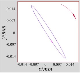
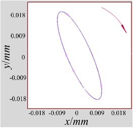
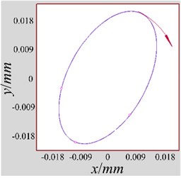
According to the Ref. [6], the shape of shaft orbit changes with different severity of fault. Fig. 2 shows shaft orbits in different degree of misalignment faults. In the condition of Fig. 2(a), the shaft orbit is an elliptical shape close to a circle, which corresponds to light fault, and there is no preload. In the condition of Fig. 2(b), the shaft orbit is a flat ellipse, which corresponds to medium fault, and there is some preload. In the condition of Fig. 2(c), the shaft orbit is outer ‘8’ shape, which corresponds to serious fault, and there is large preload.
Fig. 2Shaft orbits in different degree of misalignment faults

a)

b)

c)
From the perspective of the fault degree, Fig. 2(b) are more serious than Fig. 2(a). From the perspective of the change in curvature, Fig. 2(b) is greater than that of Fig. 2(a). The change in curvature of the shaft orbit reflects the intensity of position change of the shaft and the severity of the fault. Therefore, five indicators that reflect the change in curvature are proposed in this paper to subdivide the shaft orbits shape in Table 1, and the indicators are the slenderness , which corresponds to the elliptical shaft orbit, the bending , the ring width ratio , the angle span ratio , and the minimum radius of curvature . The slenderness is corresponding to the elliptical shaft orbit, and the bending is corresponding to the banana-shaped shaft orbit, and the ring width ratio is corresponding to the outer “8” shaft orbit, and the angle span ratio is corresponding to the inner “8” shaft orbit, and the minimum radius of curvature is corresponding to the petal-shaped shaft orbit.
Table 1 shows the corresponding relationship between shaft orbit shapes and the fault types [5]. The shaft orbits are simulated according to [12], and a series of variables are introduced to refine the classification of different shaft orbits.
Table 1The corresponding relationship between the shaft orbits and the fault types
Fault types | Shapes of shaft orbits |
Unbalance | Ellipse |
Misalignment | Banana |
Misalignment | Outer ‘8’ |
Oil whip | Inner ‘8’ |
Oil whirl | Petal |
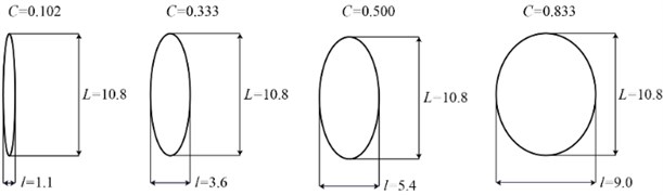
(1) The slenderness is defined as , where and represent the short and long axes of the graph, respectively. When the graph is an ellipse, the smaller is, the slimmer the ellipse is. When the graph is circular, 1. The smaller the slenderness is, the more serious the shaft vibration is, so the more serious the shaft unbalance is. Fig. 3 shows some shaft orbits with different slenderness. The slenderness of elliptical shaft orbits is in the range of 0.1 to 1, and elliptical shaft orbits are divided into three parts according to slenderness . The elliptical shaft orbit represents serious fault when the slenderness is in the range of 0.1 to 0.4, it represents medium fault when the slenderness is in the range of 0.4 to 0.7, and it represents slight fault when the slenderness is in the range of 0.7 to 1.
Fig. 3Part shaft orbits with different slenderness
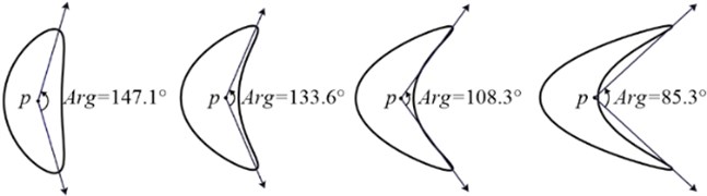
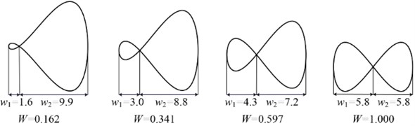
(2) The bending is defined as the angle between two lines connecting the centroid of the graph and two “vertices”. The smaller the is, the greater the bending is and the more serious the fault is. As shown in Fig. 4, with the decrease of of the banana-shaped shaft orbit, the severity degree of shaft misalignment increases. The bending of banana-shaped shaft orbits is in the range of 70° to 160°, and banana-shaped shaft orbits are divided into three according to . The banana-shaped shaft orbit represents serious fault when the bending is in the range of 70° to 100°, it represents medium fault when the bending is in the range of 100° to 130°, and it represents slight fault when the bending is in the range of 130° to 160°.
Fig. 4Part shaft orbits with different bending
(3) The ring width ratio is defined as , where and are the widths of small and large rings, respectively. The characteristic parameters are mainly applicable to the outer “8” shapes. The smaller the is, the larger the gap between the two rings is, which means that the more serious the changes in the phase of the small ring is, the more serious the fault is. Fig. 5 shows some shaft orbits with different ring width ratio . increases from left to right, and the severity of fault decreases instead. The ring width ratio of outer “8” shaft orbits are in the range of 0.1 to 1, and outer “8” shaft orbits are divided into three parts according to . The outer “8” shaft orbit represents serious fault when the ring width ratio is in the range of 0.1 to 0.4, it represents medium fault when the ring width ratio is in the range of 0.4 to 0.7, and it represents slight fault when the ring width ratio is in the range of 0.7 to 1.
Fig. 5Part shaft orbits with different ring width ratio
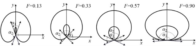
(4) The angle span ratio is defined as , where and are small and big angle at the intersection of the graph, respectively. The smaller the is, the steeper the phase change is at the intersection of inner “8” shaft orbit, and the more serious the fault is. Fig. 6 shows some shaft orbits with different angle span ratio . increases from left to right, and the severity degree of fault decreases. The angle span ratio of inner “8” shaft orbits are in the range of 0.1 to 1, and inner “8” shaft orbits are divided into three parts according to the angle span ratio. The inner “8” shaft orbit represents serious fault when the angle span ratio is in the range of 0.1 to 0.4, it represents medium fault when the angle span ratio is in the range of 0.4 to 0.7, and it represents slight fault when the angle span ratio is in the range of 0.7 to 1.
Fig. 6Part shaft orbits with different angle span ratio
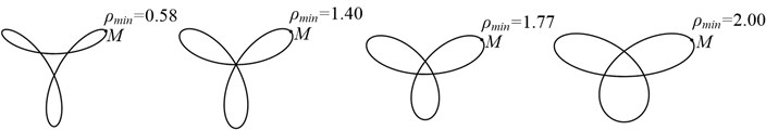
(5) The minimum curvature radius is used as a parameter to describe the degree of fault corresponding to petal-shaped shaft orbit. The point with the smallest curvature radius on the shaft orbit represents the most violent phase of the shaft. The smaller the value of is, the more serious the failure is. Fig. 7 shows some shaft orbits with different minimum radius of curvature, and the point in the Fig. 7 is the point with the smallest curvature radius. increases sequentially from left to right, and the severity of oil whip decreases. The minimum radius of curvature of petal-shaped shaft orbits are in the range of 0.5 to 2.9, and petal-shaped shaft orbits are divided into three parts according to minimum curvature radius. The petal-shaped shaft orbit represents serious fault when the minimum curvature radius is in the range of 0.5 to 1.3, it represents medium fault when the minimum curvature radius is in the range of 1.3 to 2.1, and it represents slight fault when the minimum curvature radius is in the range of 2.1 to 2.9.
Fig. 7Part shaft orbits with different minimum radius of curvature
2.1.2. Constructing a simulation dataset of fine-grained shaft orbit
According to theory of fine-grained shaft orbits, each type of shaft orbits in Table 1 is subdivided into slight, medium, and serious levels by fault feature parameters. Five types of shaft orbits are further subdivided into 15 subtypes of shaft orbits with different degrees. 500 graphs for each subtype of shaft orbits are simulated, 300 of which are randomly selected for training and the remaining 200 are used for testing. Part of the simulation dataset for fine-grained shaft orbits are shown in Table 2.
2.2. Identification method of fine-grained shaft orbits based on improved LeNet-5
In recent years, CNN has been widely used in object recognition, detection, and scene understanding [22]. CNN makes it possible to design an end-to-end deep network for identification of shaft orbits. It automatically abstracts the features suitable for classification from the images of shaft orbits, thus avoiding complex process of the traditional feature extraction. LeNet-5 [23] is a classic CNN structure and successfully applied in hand-written digital character recognition, which is a good reference for the identification of fine-grained shaft orbits. In this section, we proposed a CNN-based approach for identification of fine-grained shaft orbits by optimizing the network structure of LeNet-5.
Table 2Part of the simulation dataset for fine-grained shaft orbits
Shape of shaft orbit | Serious | Medium | Slight |
Ellipse |  |  |  |
Banana |  |  |  |
Inner “8” |  |  |  |
Outer “8” |  |  |  |
Petal |  |  |  |
Excluding the input and output layers, LeNet-5 includes 6 layers: three convolutional layers (namely C1, C3 and C5), two pooling layers (namely S2 and S4), and one fully-connected layer (namely F6). Its input image size is set to 32 × 32, and it has ten nodes corresponding to ten kinds of numbers in MNIST dataset. The kernel size in convolutional layers is fixed to 5 × 5, and in sub-sampling layer the size is 2 × 2. There are 6, 16 and 120 kernels in convolutional layers C1, C3 and C5, respectively. And there are 6 and 16 kernels in sub-sampling layers S2 and S4, respectively. The number of nodes in fully-connected layer F6 is set as 84.
Convolutional layers are used for feature extraction in CNN. The design of the convolutional layer structure mainly includes four parts: the choice of activation function, the number of convolutional layers, the size and number of convolution kernels. Since the size of input image is only 32×32, the range of the number of convolutional layers, pooling layers and fully-connected layers is from 1 to 3, and the size of convolutional kernels are selected among 3×3, 4×4 and 5×5. The number of convolutional kernels determines the number of linear combinations of network and the ability to extract features. It usually has a wide range from 12 to 512. As for the activation function, it improves the network’s ability of building nonlinear models, and directly affects the convergence speed and recognition rate of CNN. The performance of different active functions in CNN is discussed in Ref. [24, 25]. It is found that there is a problem of gradient disappearance in saturating nonlinear functions. The unsaturated nonlinear function can not only solve those problems, but also accelerate the convergence speed and improve the performance of CNN [25-27]. Therefore, the appropriate activation function in this paper is selected among Softplus, LReLU, PReLU, RReLU and ELU functions.
Table 3Range of tested hyperparameters
Hyperparameters | Range |
Number of convolutional layers | 1, 2, 3 |
Number of pooling layers | 1, 2, 3 |
Number of fully-connected layers | 1, 2, 3 |
Size of convolutional kernels | 3×3, 4×4, 5×5 |
Number of convolutional kernels | 12, 16, 20, 32, 64, 128, 160, 192, 256, 512 |
Number of nodes of fully-connected layers | 30, 84, 120 |
Pooling method | Max pooling, Mean pooling |
Active function | ReLU, Softplus, LReLU, PReLU, RReLU, ELU |
Optimizer | SGD, Adam, Adadelta, RMSprop |
With the advent of various optimization methods, such as adaptive moment estimation (Adam), modified adaptive gradient (Adadelta), root-mean-square propagation (RMSprop), etc., it is possible to adjust parameters (weights and biases) during training adaptively [28, 29]. They can mitigate the influence of two changes of gradient descent: the local minimum trap and choosing an appropriate learning rate [29]. Therefore, the optimizer in this paper are selected among stochastic gradient descent (SGD), Adam, Adadelta, and RMSprop.
The range of tested hyperparamenters are shown in Table 3. The hyperparameters of the optimal CNN for the identification of fine-grained shaft orbits are selected by experiments in Section 3.1.
3. Experiment on the identification of fine-grained shaft orbits
Firstly, this section establishes a new CNN that is most suitable for the identification of fine-grained shaft orbits through optimizing the follow parameters: the number of convolutional layers and fully connected layers, the number and the size of convolution kernel, the nodes number of each fully connected layers, pooling method and optimizer. Secondly, experiments on simulation dataset and measured dataset is designed to prove that the proposed method is suitable for the identification of fine-grained shaft orbits.
3.1. The structure of optimized LeNet-5 for identification of fine-grained shaft orbits
Since LeNet-5 is specifically designed for hand-written digits, it differs from the identification of shaft orbits in this paper. Therefore, some preliminary improvements have been made as follows:
(1) The number of feature maps determines the number of linear combinations for network and the ability of features extraction. To improve that, the numbers of feature maps for the first and second pairs of convolution and pooling layers: C1/S2 and C3/S4, are all changed to 12. After adjustment, the total number of linear combinations of the CNN network is increased from 6 by 16 to 12 by 12.
(2) LeNet-5 has a large number of parameters in the fully connected layer, which greatly increases the complexity of the network and the training time. And network with many parameters are easily overfitted when the data is insufficient. Therefore, only one full connection layer is retained in the primary improved LeNet-5.
(3) The Sigmoid active function applied in LeNet-5 is not universal, and it is found that there is a problem of gradient disappearance in Sigmoid functions. ReLU function can overcome that problem and it has a much faster convergence speed than Sigmoid functions. In Ref. [26, 27], ReLU function are all adopted in convolution layers. Hence the ReLU function is selected as the active function in the primary improved LeNet-5.
(4) The number of nodes in full connection layer F6 is replaced with 15 to correspond to 15 kinds different fine-grained shaft orbits.
(5) SGD in CNN usually faces two challenges: the choice of an appropriate learning rate and how to avoid local minimum trap [28, 29]. Ref [29] has proved that RMSprop is better than SGD in some respects. Hence RMSprop is selected to be the optimizer in the primary improved LeNet-5.
After the primary improvement, the network obtains a recognition rate of 93.20 %, and the training parameters of the network are set as follows: the training period is 3000; the batch size is 64; the initial learning rate is 0.0001. Although there is some improvement on the recognition rate, there is still room for further improvement. In order to find the optimal CNN network for the identification of the fine-grained shaft orbits, the hyperparameters of CNN network will be optimized in terms of the number of convolution layers, the number and the size of convolutional kernels, the number of fully connected layers, the number of nodes in each fully connected layer, the active function used in convolutional layers, the pooling method and the optimizer.
3.1.1. Numbers of convolutional layers and pooling layers
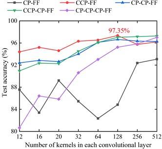
The structure of the convolutional layer and the pooling layer directly determine the feature extraction ability of CNN. It mainly includes four part: the numbers of convolutional layers, pooling layers, convolutional kernels, and the size of the convolutional kernel. The optimal numbers of convolutional layers and pooling layers are first obtained by experiments, the result of experiments is shown in Fig. 8, where the C means the convolutional layers, the P means pooping layer, and the F means the fully-connected layer. The numbers of kernels in each convolutional layers are set to be the same. In the CP-FF, CCP-FF, CP-CP-FF and CCP-CP-FF structure, the size of convolutional kernels is all set to 5×5. Due to the limitation of the network structure, the size of convolutional kernels in CP-CP-CP-FF structure is set to 3×3. The unspecified parameters of the network are the same as those of the primary improved LeNet-5.
It can be seen from Fig. 8 that the test accuracy of the CCP-FF network changes little and can reach the highest 97.35 % when the number of convolution kernel is set to be 128. Therefore, the CNN structure is set to be CCP-FF, which includes two convolutional layers and one pooling layer for the following experiments.
Fig. 8The test accuracy of different CNN structure with different convolutional kernels: the C means the convolutional layers, the P means pooping layer, and the F means the fully-connected layer
3.1.2. The number and size of kernels in each convolutional layer
The numbers of kernels in convolutional layers are also important for CNN. 9 groups of contrast experiments are conducted to find the optimal parameters, and the results of experiments are shown in Table 4. The test accuracy of the network reaches the highest 97.44 % when the numbers of kernels of the first and second convolutional layers are 96 and 192, respectively. It shows that it has a more comprehensive extraction performance for fine-grained shaft orbits. Therefore, the numbers of kernels of the first and second convolutional layers in this paper are set to 96 and 192 for the following experiments.
The size of the kernels is another important parameter of the convolutional layer. The experimental results of nine different kernel size are shown in Table 5. It shows that the most suitable sizes of kernels of the first and second convolutional layers are 5×5 and 4×4, respectively.
3.1.3. The structure of fully-connected layers
The structure of the fully connected layer mainly includes the number of fully-connected layers and the number of nodes of each layer. Four comparative experiments are conducted, and the experimental result is shown in Table 6. It indicates that three fully-connected layers are suitable for identification of fine-grained shaft orbits, and the numbers of each layer’s nodes are 120, 84 and 30, respectively.
Table 4The identification results of CCP-FF network with different numbers of convolutional kernels
Numbers of kernels of the first and second convolutional layers | Train time (s) | Test time (s) | Train accuracy | Test accuracy |
64,128 | 175.44 | 1.08 | 100 % | 97.33 % |
64,160 | 192.56 | 1.16 | 100 % | 97.24 % |
64,192 | 211.73 | 1.21 | 100 % | 97.37 % |
96,128 | 199.85 | 1.21 | 100 % | 97.28 % |
96,160 | 220.15 | 1.29 | 100 % | 97.18 % |
96,192 | 243.60 | 1.39 | 100 % | 97.44 % |
128,128 | 222.28 | 1.35 | 100 % | 97.35 % |
128,160 | 248.88 | 1.44 | 100 % | 97.30 % |
128,192 | 275.33 | 1.48 | 100 % | 97.32 % |
Table 5The identification results of CCP-FF network with different size of convolutional kernels
The size of kernels of the first and second convolutional layers | Train time (s) | Test time (s) | Train accuracy | Test accuracy |
5×5, 5×5 | 243.60 | 1.39 | 100 % | 97.44 % |
5×5, 4×4 | 250.65 | 1.38 | 100 % | 97.49 % |
5×5, 3×3 | 257.57 | 1.46 | 98.63 % | 96.97 % |
4×4, 5×5 | 305.69 | 1.43 | 98.44 % | 96.82 % |
4×4, 4×4 | 256.67 | 1.46 | 99.48 % | 97.45 % |
4×4, 3×3 | 258.90 | 1.42 | 99.22 % | 97.15 % |
3×3, 5×5 | 319.49 | 1.37 | 98.44 % | 96.13 % |
3×3, 4×4 | 320.27 | 1.61 | 100 % | 96.91 % |
3×3, 3×3 | 269.57 | 1.50 | 99.48 % | 96.66 % |
Table 6The identification results of CCP-FF network with different structure of fully-connected layers
The number of fully-connected layers | The number of nodes of each fully-connected layer | Train time (s) | Test time (s) | Test accuracy |
1 | 84 | 226.80 | 1.40 | 96.13 % |
1 | 120 | 238.50 | 1.39 | 96.93 % |
2 | 120, 84 | 250.65 | 1.38 | 97.49 % |
3 | 120, 84, 30 | 249.97 | 1.45 | 97.61 % |
3.1.4. Optimizer
SGD, Adam, Adadelta, RMSprop are compare in the flowing experiments to select the optimal optimizer of proposed CNN, and the experimental results are shown in Fig. 9. The best test accuracy of SGD, Adam, Adadelta, and RMSprop are 97.75 %, 97.96 %, 97.92 %, and 97.61 %, respectively. The four methods can all achieve a very high test accuracy, among which the Adam method has the highest test accuracy. At the meantime, as can be seen from Fig. 9, the Adam method has the highest convergence rate. Therefore, Adam method is selected to be the optimizer of CNN in this paper.
3.1.5. The optimal structure of CNN for the identification of fine-grained shaft orbits
Several experiments are carried out in order to find the optimal activation function and pooling method. Activation function include ReLU, Softplus, LReLU, PReLU, RReLU, ELU and pooling method include max pooling and mean pooling. The experimental result indicates the most suitable activation function is ReLU function and the most suitable pooling method is max pooling. Therefore, the final optimal structure of CNN proposed in this paper is determined, which is shown in Fig. 10. It includes the input layer, two convolutional layers, one pooling layer, three fully-connected layers and the output layers. The optimizer of the optimal structure of CNN is Adam method. The parameters of each layer s are shown in Table 7.
Fig. 9Experimental results of different optimizers
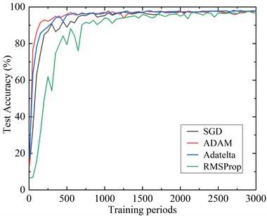
Fig. 10The structure of the optimal structure of CNN for the identification of fine-grained shaft orbits
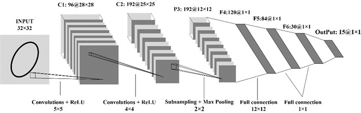
Table 7The parameters of each layer in the optimal structure of CNN for the identification of fine-grained shaft orbits
Layer number | Layer type | The size of kernel | The number of feature maps | The size of feature maps |
C1 | Convolutional layer | 5×5 | 96 | 28×28 |
C2 | Convolutional layer | 4×4 | 192 | 25×25 |
P3 | Pooling layer | 2×2 | 192 | 12×12 |
F4 | Fully-connected layer | 12×12 | 120 | 1×1 |
F5 | Fully-connected layer | 1×1 | 84 | 1×1 |
F6 | Fully-connected layer | 1×1 | 30 | 1×1 |
Output | Output layer | 1×1 | 15 | 1×1 |
3.2. The experiment on the identification of simulated fine-grained shaft orbits
To further highlight the advantages of the improved CNN on fine-grained shaft orbits classification, several traditional methods are compared. The height function (HF) [30], shape context (SC) [31] and inner distance shape context (IDSC) [32] are selected as shape descriptors to extract the features of shaft orbits, and BP neural network and SVM [7] are used as classifiers. All shape descriptors selected 60 feature points as samples. The parameters of SVM are set as follows: the “linear kernel function” is selected and the other parameters are the default. The parameters of BP neural network in MATLAB toolbox are set as follows: the period is set to 1000, the target error is set to 0.0001, the node number of hidden layer is set to 100, S-type function “logsig” is selected as the excitation function, and linear function “Purelin” is adopted as the output layer excitation function. The experimental results of are shown in Table 8. The results are the average of 20 trials.
Table 8Results of the recognition on 15 kinds of fine-grained shaft orbits using different methods
Methods | The average recognition rate | Training period | Training time (s) | Single sample testing time (ms) |
HF+BP | 81.50 % | 1000 | 231.09 | 19.11 |
HF+SVM | 81.61 % | – | 114.30 | 31.17 |
IDSC+BP | 77.20 % | 1000 | 486.71 | 61.13 |
IDSC+SVM | 86.08 % | – | 319.20 | 96.71 |
SC+BP | 71.86 % | 1000 | 361.53 | 35.49 |
SC+SVM | 87.67 % | – | 208.11 | 67.49 |
Primary improved LeNet-5 | 93.20 % | 3000 | 75.54 | 0.06 |
Optimized LeNet-5 | 97.96 % | 3000 | 249.97 | 0.16 |
It can be seen from the Table 8 that the average recognition rate of the optimized LeNet-5 method proposed in this paper is the highest 97.96 %, which is much higher than that of traditional methods. In addition, the recognition rate of optimized LeNet-5 method is 4.76 % higher than that of the primary improved LeNet-5 network method. In single sample testing time, the optimized LeNet-5 method is much better than the traditional methods. Although the recognition speed of the proposed method is slightly lower than that of the primary improved LeNet-5 network, the test time of a single sample of optimized LeNet-5 method only needs 0.16 milliseconds, which can still meet the real-time performance of the identification.
Although the training time of the optimized LeNet-5 network is longer than that of the primary improved LeNet-5 method and the traditional methods. In practice, the training process can be completed ahead of time, so the real-time performance of the algorithm is not affected.
Therefore, the method proposed in this paper has the best performance, its average time for identifying a shaft orbit is only 0.16 milliseconds and the average recognition rate can reach 97.96 %.
3.3. Experiments on the identification of measured fine-grained shaft orbits
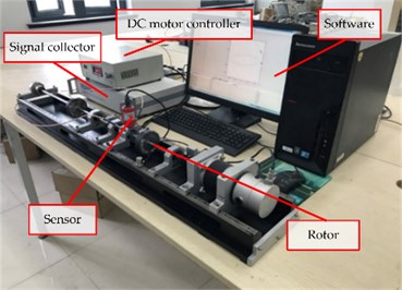
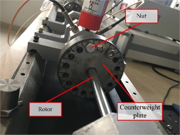
The testing bench of rotor (STS1000 online vibration monitoring and analysis system) is used to further verify the practicability of the algorithm, as showed in Fig. 11. The testing bench includes one bearing rotor, several displacement sensors, one signal acquisition unit, one DC motor controller and testing software, etc. The details of the sensors in the testing bench are shown in Table 9. Different degrees of faults for shaft imbalance are generated by adding different amounts of nuts to the counterweight plate and changing the speed of shaft.
Table 9The details of the sensors in the testing bench
Name | Sensitivity | Frequency range | Measuring range | Measuring conditions |
Magnet-electrical absolute vibration velocity transducer | 28 mv/mm/s | 10 Hz-1000 Hz | 0-10 mm/s (Less than 80 Hz) | No strong electromagnetic interference, –30 ℃ - +80 ℃ |
Piezoelectric vibration acceleration transducer | 98.5 mv/g | 0.5 Hz-10000 Hz | ± 50 g | –50 ℃ - +120 ℃ |
Eddy current vibration displacement pickup | 8 mv/um | 0 Hz-4000 Hz | 1.8 mm | –30 ℃ - +120 ℃ |
Using the slenderness presented in Section 2.1 as the indicator, 900 different measured elliptical shaft orbits of different severity are selected in the collected shaft orbits by the testing bench, which include 300 serious, 300 medium and 300 slight faults, respectively. And part of the measured fine-grained shaft orbits of different unbalance faults are shown in Fig. 12. Two-thirds of measured shaft orbits replace elliptical shaft orbits in simulated training dataset to train the optimized LeNet-5 proposed in this paper. And the remaining one third of measured shaft orbits are used for identification to further verify the practicability of the method proposed in this paper. Similar to section 3.1, the primary improved method and the traditional methods are used to set comparative experiments, in which the trained BP networks or SVM models of each method in Section 3.2 are used to identify 300 measured shaft orbits.
Fig. 11Rotor testing bench: a) testing bench; b) counterweight plate
a)
b)
Fig. 12The measured fine-grained shaft orbits of different unbalance faults: a) serious; b) medium; c) slighter
a)
b)
c)
The optimized LeNet-5 is used to test the measured different fine-grained shaft orbits, and the results are shown in Table 10. The networks or SVM models used in the measured experiments are all trained in section 3.2, so the training results are the same as in Table 8, which are not listed in Table 10.
By comparing experimental results on simulated shaft orbits and actual measured shaft orbits in Table 8 and Table 10, the accuracy of identification on the measured data is lower than the simulation data shaft orbit with the same algorithm. This is because measured shaft orbits are more complex than simulated shaft orbits. However, the reduction in the accuracies of the method proposed in this paper is small, not exceeding 0.82 %. It shows that the method proposed in this paper have a great practical performance.
Similar to the analysis of simulation result in section 3.2, the following conclusions can be drawn:
(1) From the perspective of the average recognition rate, the method proposed in this paper is more suitable for identification on actual measured shaft orbit than the primary improved method and the traditional methods.
(2) From the perspective of the single sample testing time, the performance of the method proposed in this paper are much better than the traditional methods.
Table 10Identification result of the measured fine-grained shaft orbits for shaft unbalance faults
Methods | The average recognition rate | Single sample testing time (ms) |
HF+BP | 80.75 % | 20.52 |
HF+SVM | 80.83 % | 32.94 |
IDSC+BP | 75.86 % | 63.67 |
IDSC+SVM | 84.91 % | 98.11 |
SC+BP | 69.93 % | 36.51 |
SC+SVM | 85.82 % | 69.15 |
Primary improved LeNet-5 | 91.53 % | 0.07 |
optimized LeNet-5 | 97.14 % | 0.17 |
4. Conclusions
This paper proposes a new deep learning-based fault diagnose method for rotating machinery. The proposed method judges the type and severity of the fault by identification the shape of shaft orbit. A new theory of fine-grained shaft orbit is proposed to divide different shaft orbits into several subclasses that can reflect the severity of the fault, and the appropriate network structure of CNN is designed to identify the fine-grained shaft orbits. The recognition accuracy and real-time performance of the proposed method are verified by a series of contrast experiments. The experimental results show that the proposed method can reach 97.69 % and 97.14 % in the simulated and measured fined-grained shaft orbit dataset, respectively, and the test time of each sample is less than 0.17 ms. It is demonstrated that the proposed method is far superior to the existing traditional algorithms in effectiveness and accuracy and can provide some guidance and support for fault diagnosis of rotating machinery.
References
-
Zhang X., Zhou J., Guo J., Zou Q., Huang Z. Vibrant fault diagnosis for hydroelectric generator units with a new combination of rough sets and support vector machine. Expert Systems with Applications, Vol. 39, Issue 3, 2012, p. 2621-2628.
-
Chen X., Zhou J., Xiao H., Wang E., Xiao J., Zhang H. Fault diagnosis based on comprehensive geometric characteristic and probability neural network. Applied Mathematics and Computation, Vol. 230, Issue 3, 2014, p. 542-554.
-
Xu F., Tse W. T. P., Tse Y. L. Roller bearing fault diagnosis using stacked denoising auto encoder in deep learning and Gath-Geva clustering algorithm without principal component analysis and data label. Applied Soft Computing Journal, Vol. 73, 2018, p. 898-913.
-
Xiang X., Zhou J., Yang J., Liu L., An X., Li C. Mechanic signal analysis based on the Haar-type orthogonal matrix. Expert Systems with Applications, Vol. 36, Issue 6, 2009, p. 9674-9677.
-
Sun H. F., Pan L. P., Zhang F., Cao D. F. Review of identification of shaft orbit for rotating machinery. Journal of China Institute of Water Resources and Hydropower Research, Vol. 12, Issue 1, 2014, p. 86-92.
-
Jiang Z., Li Y. Research on feature extraction of shaft orbit for rotating machine. Journal of Vibration, Measurement and Diagnosis, Vol. 27, Issue 2, 2007, p. 98-101.
-
Fu B., Zhou J. Z., Chen W. Q., Yu B. H. Identification of the shaft orbits for turbine rotor by modified Fourier descriptors. Proceedings of Third International Conference on Machine Learning and Cybernetics, 2004, p. 1162-1167.
-
Wang C., Zhou J., Kou P, Lou Z., Zhang Y. Identification of shaft orbit for hydraulic generator unit using chain code and probability neural network. Applied Soft Computing, Vol. 12, Issue 1, 2012, p. 423-429.
-
Xiang X., Zhou J., An X., Peng B., Yang J. Fault diagnosis based on Walsh transform and support vector machine. Mechanical Systems and Signal Processing, Vol. 22, Issue 7, 2008, p. 1685-1693.
-
Yan C., Zhang H., Li H., Yang L., Huang W. Automatic identification of shaft orbits for steam turbine generator sets. WRI Global Congress on Intelligent Systems, 2009.
-
Bao J., Zhu Z., Tang H., Lu T., Zhang Q. Apply low-level image feature representation and classification method to identifying shaft orbit of hydropower unit. 6th International Conference on Intelligent Human-Machine Systems and Cybernetics, 2014.
-
Wu B., Feng S., Sun G., Xu L., Ai C. Identification method of shaft orbit in rotating machines based on accurate Fourier height functions descriptors. Shock and Vibration, 2018.
-
Tra V., Kim J., Khan S. A., Kim J. Bearing fault diagnosis under variable speed using convolutional neural networks and the stochastic diagonal Levenberg-Marquardt algorithm. Sensors, Vol. 17, Issue 12, 2017, p. 2834.
-
Guo Sheng., Yang T., Gao W., Zhang C. A novel fault diagnosis method for rotating machinery based on a convolutional neural network. Sensors, Vol. 18, Issue 5, 2018, p. 1429.
-
Yu W., Huang S., Xiao W. Fault diagnosis based on an approach combining a spectrogram and a convolutional neural network with application to a wind turbine system. Energies, Vol. 11, Issue 10, 2018, p. 1-11.
-
Guo S., Yang T., Gao W., Zhang C., Zhang Y. An intelligent fault diagnosis method for bearings with variable rotating speed based on pythagorean spatial pyramid pooling CNN. Sensors, Vol. 18, Issue 11, 2018, p. 3857.
-
Xu G., Liu M., Jiang Z., Söffker D., Shen W. Bearing fault diagnosis method based on deep convolutional neural network and random forest ensemble learning. Sensors, Vol. 19, Issue 5, 2019, p. 1088.
-
Lu C., Wang Z., Zhou B. Intelligent fault diagnosis of rolling bearing using hierarchical convolutional network based health state classification. Advanced Engineering Informatics, Vol. 32, 2017, p. 139-151.
-
Hoang, D., Kang, H. Rolling element bearing fault diagnosis using convolutional neural network and vibration image. Cognitive Systems Research, Vol. 53, 2019, p. 42-50.
-
Wang F., Jiang H., Shao H., Duan W., Wu S. An adaptive deep convolutional neural network for rolling bearing fault diagnosis. Measurement Science and Technology, Vol. 28, Issue 9, 2017, p. 095005.
-
Guo L., Lei Y., Li N., Yan T., Li N. Machinery health indicator construction based on convolutional neural networks considering trend burr. Neurocomputing, Vol. 292, Issue 31, 2018, p. 142-150.
-
Sun W. F., Yao B., Chen B. Q., He Y. C., Cao X. C., Zhou T. X., Liu H. G. Noncontact surface roughness estimation using 2d complex wavelet enhanced ResNet for intelligent evaluation of milled metal surface quality. Applied Sciences, Vol. 8, Issue 3, 2018, p. 381.
-
LeCun Y., Bottou L., Bengio Y., Haffner P. Gradient-based learning applied to document recognition. Proceedings of the IEEE, Vol. 86, Issue 11, 1998, p. 2278-2323.
-
Krizhevsky A., Sutskever I. I., Hinton G. ImageNet classification with deep convolutional neural networks. Proceedings of the Advances in Neural Information Processing Systems, 2012, p. 1097-1105.
-
Wei G. F., Li., G., Zhao J., He A. X. Development of a LeNet-5 gas identification CNN structure for electronic noses. Sensors, Vol. 19, Issue 1, 2019, p. 217.
-
Nair V., Hinton G. E., Farabet C. Rectified linear units improve restricted Boltzmann machines. Proceedings of the 27th International Conference on Machine Learning, 2010, p. 807-814.
-
Boureau Y., Roux N. L., Bach F., Ponce J., LeCun Y. Ask the locals: Multi-way local pooling forimage recognition. Proceedings of the International Conference on Computer Vision, 2011, p. 2651-2658.
-
Ruder S. An Overview of Gradient Descent Optimization Algorithms. CoRR, abs/1609.04747, 2016.
-
Vijayashanthar V., Qiao J., Zhu Z., Entwistle P., Yu G. Modeling fecal indicator bacteria in urban waterways using artificial neural networks. Journal of Environmental Engineering, Vol. 144, Issue 6, 2018, https://doi.org/10.1061/(ASCE)EE.1943-7870.0001377.
-
Wang J. W., Bai X., You X. G., Liu W. Y., Latecki L. J. Shape matching and classification using height functions. Pattern Recognition Letters, Vol. 33, Issue 33, 2012, p. 134-143.
-
Belongie S., Malik J., Puzicha J. Shape matching and object recognition using shape contexts. IEEE Transactions on Pattern Analysis and Machine Intelligence, Vol. 24, Issue 4, 2002, p. 509-522.
-
Ling H. L. H., Jacobs D. W. Shape classification using the inner-distance. IEEE Transactions on Pattern Analysis and Machine Intelligence, Vol. 29, Issue 2, 2007, p. 286-299.
Cited by
About this article

This research was funded by the National Natural Science Foundation of China (Grant Nos. 51775177, 51675166) and Natural Science Foundation of Shanghai (Grant No. 19ZR1463800).
Bo Wu designed the methods. Songlin Feng collected relevant literature. Guodong Sun analyzed experimental data. Liang Xu wrote the paper. Chenghan Ai checked the grammar of the paper. All of the authors participated in the project, and they read and approved the final manuscript.
