Abstract
Randomness complexity is a kind of features which is widely used to describe bearings’ degradation. However, different randomness complexities present different properties. It is necessary to figure out different randomness complexities’ properties. In this paper, we are going to make comparisons of seven commonly used randomness complexities namely approximate entropy, sample entropy, fuzzy entropy, Shannon entropy, permutation entropy, Lempel-Ziv complexity and complexity by simulation signals with three different aspects and two run-to-failure bearing’s data. By comparisons, we have found that there are a kind of similarity between them and we have proposed a trend similarity index to expound this similarity. Based on the comparisons, we can infer that randomness complexities are a family feature of rolling bearings’ degradation. Among the seven discussed complexities, sample entropy has the best performance, and it can be a good representative of the complexity features. In this paper, the difference between complexity features and other features when monitoring bearings’ degradation have been discussed. The research will provide a reference for rolling bearings’ multi-features dimensionality reduction by attribute selection method.
Highlights
- There are a kind of similarity between different randomness complexity.
- A new similarity index is proposed to expound the trend similarity.
- Simulation signals with three different aspects are used for comparisons.
- For the seven randomness complexities in the paper, sample entropy has the best performance.
1. Introduction
The rolling bearing is one of the most frequently used components in rotating machinery, which has an important influence on the modern industry. The function of bearings is to permit linear motion or constrained relative rotation between two parts. During the operation, the bearings are often subject to high loading and severe conditions. Under this severe operating condition, defects are often developed on the bearing components which are the most frequent cause of failure in mechanisms [1]. Most of the operational life of a bearing shows no significant trend until the time very close to failure [2]. Hence, it is pivotal and cost-effective to find suitable methods to detect fault and monitor the degradation process [3]. So, the condition-based monitoring (CBM) have come into being, and the industry is undergoing the transition from time-based part replacement decisions in operational systems to CBM [4]. The most extensively used monitoring tool is vibration signal. As a result, a plethora of methods for diagnosing bearing faults have been proposed, good reviews can be seen in Ref. [5-9]. Although to detect faults effectively, these features can hardly describe the degradation of bearings, let alone estimate the remaining useful life (RUL) of bearings. For instance, two main families of signal processing tools have gained a leading role in the diagnostic of such components: the kurtogram-based family and the cyclostationarity family [10], but both of them can hardly extract indicators for degradation process. Many references used statistical parameters such as root mean square (RMS), kurtosis and crest factor as the degradation indicators, but neither of them always shows an increasing trend during the degradation process. To find a reliable, robust, trend consistent feature, and meanwhile, which can clearly reflect the stage of the degradation is all-important.
Complexity is a kind of features which have been widely used in many areas for decades. Rapp and Schmah [11, 12] have classified a variety of complexity algorithms into two categories. One is the randomness complexity, the other is the rule complexity. For example, language is complex, if a meaningful sentence is randomly disturbed, the original text should have higher rule complexity but lower randomness complexity. The “snow” displayed on television when there is no signal presents high randomness complexity but low rule complexity. Boskoski et al. have presented a kind of rule complexity in Ref. [2]. They supposed that both periodical and purely random signals should have no complexity. The complex signals should be located somewhere in between and have chaotic behaviors. And they have defined the product of Rényi entropy and Jensen-Rényi divergence as a rule complexity.
Compared to the rule complexity, randomness complexity is more common used and easy to realize. Many references have used randomness complexities for diagnosis and prognostics. Ref. [13] proposed a quantitative diagnosis method of a spall-like fault for bearings based on empirical mode decomposition (EMD) and approximate entropy (ApEn). Ref. [14] proposed a bearing diagnosis method based on EMD energy entropy and ANN. Ref. [15] presented a bearing diagnosis approach based on local characteristic-scale decomposition (LCD) and fuzzy entropy (FuzzyEn). Spectral entropy has been applied as a complementary index of bearings for performance degradation assessment in Ref. [16]. Yan et al. have applied Lempel-Ziv complexity (LZC), ApEn and permutation entropy (PermEn) as features for bearings diagnosis, respectively in Ref. [17-19]. Shannon entropy (ShEn) is selected as one of the basic features for prognostics in Ref. [20]. A bearing diagnosis method based on empirical wavelet transform and fuzzy entropy is proposed in Ref. [21]. Zhao et al. have applied Multi-scale Fuzzy Entropy and EEMD for motor bearings [22]. General mathematical morphological particle and mathematical morphological fractal dimension are respectively proposed in Ref. [23, 24]. In the numerous relevant literatures, authors have applied many randomness complexities for research and even combined with signal processing methods like EMD, LCD and wavelet transform. No matter what the forms of the randomness complexities are, the basic principle of randomness complexities is invariable, namely, the greater the regularity is, the lower the randomness complexities value. For convenience, when we talk about randomness complexity later, we use complexity instead.
The history of the complexity can be traced back to 1940s when Shannon first developed information theory and proposed Shannon entropy [25]. When calculating ShEn in frequency domain, the entropy is called spectrum entropy. A problem with the ShEn is that it is relatively insensitive to the changes in the tails of the distribution, so Rényi extended and generalized the ShEn by proposing Rényi entropy in 1961 [26]. The definition of Kolmogorov complexity (KC) is proposed by Kolmogorov in 1965, which can measure pointwise randomness. The KC is different from ShEn where it only concerned with the average information of a random source [27]. Some equivalences between ShEn and KC is discussed in Ref. [28]. In 1976, Lempel and Ziv proposed a specific algorithm for the calculation of KC called LZC [29]. In 1991, ApEn is first developed by Pincus to handle the limitations that accurate entropy calculation requires vast amounts of data and great influence by system noise [30]. Sample entropy (SampEn) is a modification of ApEn proposed by Richman and Moorman in 2000 [31]. It has two advantages over ApEn: a relatively trouble-free implementation and data length independence. Besides, SampEn needn’t the template vector comparison between itself. In Ref. [32], Costa et al. have extended SampEn named multiscale SampEn, where the SampEn is a special case of multiscale SampEn with the skipping parameter equals to one. In 2002, Bandt and Prompe introduced PermEn which based on comparisons of neighboring values of times series [33]. FuzzyEn is first proposed by Chen et al, and it extended the “membership degree” with a fuzzy function [34]. The concept of complexity () was proposed by Chen and Gu [35]. Cai and Sun [36, 37] had been improved . In literature, there are more than ten proposed complexities, and we would not enumerate them. Distinguishingly, fractal dimensions and Lyapunov exponents are specific complexities because both of them are sensitive to the noise and generally used to test chaotic behaviors. Their application is narrow, and lack of adaptability.
In this paper, we are going to explore the properties of the seven commonly used complexities, i.e., ApEn, SampEn, FuzzyEn, ShEn, PermEn, LZC, with simulation signals and run-to-failure bearing’s vibration data. After the comparisons, we have found there are some similarities within, and we have proposed an index to measure these similarities. From the comparison, we can figure out which one has the best performance. In this paper, we will engage in discussing the similarities of complexities and try to prove that complexities are a good family feature of rolling bearings’ degradation.
The paper is organized as follows. In Section 2, the calculation procedures of seven complexities are introduced. Based on their own algorithms, we have classified them into three categories and discussed them by their own definitions. The performance of complexities in simulation signals is in Section 3, and we will compare them in three different aspects. In Section 4, we are going to use two run-to-failure data (an inner race fault and an outer race fault) to examine their performance in real bearing’s data. Next, we have proposed a trend similarity index to measure the similarity between complexities. A detailed discussion is presented in Section 5. Finally, concluding remarks are given in Section 6.
2. Brief introduction of the seven complexities
Above all, we have reviewed the development of complexities. In this section, we are going to briefly introduce the calculation procedures of the seven complexity features, namely, ShEn, ApEn, SampEn, FuzzyEn, LZC and . The parameters of the features are stated as well.
2.1. Shannon entropy
ShEn is the first proposed complexity, and it quantifies the probability density function (PDF) of the signal as where is all amplitude values of the signal and is the probability that amplitude value occurs anywhere in the signal [25]. However, in the case of measured signals, the PDF is not known and should be estimated. Also, to consider all amplitude is not reasonable generally. The easy way to evaluate the PDF is to use the histogram where the amplitude range () of the signal can be divided into bins linearly so that the ratio is constant. The ratio characterizes the average filling of the histogram. It is worth to notice that there is something difference between the real PDF and the histogram. To reduce the influence, the ratio should be set bigger. However, the bigger ratio will reduce the ability of noise resistance. In this paper, we set it as 50.
2.2. Approximate entropy
The calculation steps of ApEn are as follows [30]:
Step 1: Given an point time series, and form vector sequences through , defined by These vectors represent consecutive values with th point.
Step 2: The distance between vectors and can be defined as the maximum difference in their respective scalar components, where:
Step 3: For each vector , a measure that can describe the similarity between the vector and all other vectors can be constructed as:
where is the Heaviside step function, and it is represented as:
The parameter symbolizes a tolerance value or similarity criterion, which is defined as , where is a positive constant, and is the standard deviation of the time series. The parameter is considered as a regularity or frequency of patterns similar to a given pattern of window length .
Step 4: Define and define . Given a finite time series with data points, the statistic ApEn value is defining the .
The four steps can be described as phase-space reconstruction, distance calculation, similarity calculation and complexity calculation. The concept of ApEn is derived from correlation dimension. When calculating correlation dimension, the correlation integral must be obtained first, defined as:
which is similar to . It has been proved that there is a relationship with , where is the correlation dimension. Since, can be estimated by calculating the slope of the when increasing from a small value.
2.3. Sample entropy
The calculation procedures of SampEn are as follows [31]:
Step 1 and Step2: Phase-space reconstruction and distance calculation as the same as step 1 and 2 in the calculation of ApEn.
Step 3: Given the tolerance value and count the number of as , and define , where and . Calculate the mean value as.
Step 4: Calculate, and define . The statistic SampEn value is estimated by defining the .
2.4. Fuzzy entropy
Based on the ApEn, FuzzyEn expanded the in ApEn’s third step. Heaviside step function causes a kind of two-state classifier, which is a crisp one, namely the classifier is one or the other. FuzzyEn combined fuzzy theory with ApEn. By introducing the “membership degree” with a fuzzy function which associates each point with a real number in the range [0, 1], the fuzzy theory gives a property that the higher is, the higher the membership grade of x in the relevant set. When calculating FuzzyEn, Chen et al. defined the fuzzy function as, where determines the width and the gradient of the boundary of the exponential function (It is generally set to be 2), and replace the Heaviside step function in the ApEn [34]. At last, the statistic FuzzyEn is estimated by. Moreover, FuzzyEn has a difference in distance calculation compared with ApEn. In FuzzyEn, vectors are generalized by removing the baseline of themselves.
2.5. Permutation entropy
The calculation steps of PermEn are as follows [33]:
Step 1: Phase-space reconstruction as same as step 1 in the calculation of ApEn.
Step 2: Arrange in an increasing alignment. The number of values contained in each can be arranged in an increasing alignment as:
Accordingly, any vector can be mapped onto a set of symbols as , where and . is one of the symbol permutations, which is mapped onto the number symbols in -dimensional embedding space. If are the probability distribution of each sequences where , then the PermEn for the times series of order can be defined as the Shannon entropy as for the symbol sequences:
2.6. Lempel-Ziv complexity
The calculation steps of LZC are as follows [29]:
Step 1: To calculate Lempel-Ziv complexity, the time series should be conducted “coarse-graining” operation first. In general, the time series would change to a sequence that only contains two symbols. The sequence is reconstructed by comparing the value of each sample of the previous sequence with the median value (or mean value, we take the median value as default). If the sample’s value is large than , it will change to 1, otherwise as 0.
Step 2: By obtained the two-symbol point sequence , initialize , , and . Set . Due to the does not belong to , so set , and .
Step 3: Set and judge whether the belongs to , if true, set and ; if not, then set , and . Repeat step 3 to the end of the sequence. Finally, we have the .
Step 4: The length of the sequence has obvious influence on the . So, Lempel and Ziv gave a normalized LZC, which is defined as .
2.7. complexity
The calculation steps of are as follows [36]:
Step 1: Implement Fast Fourier Transform (FFT) for the time series and gain the spectrum where .
Step 2: Obtain , where it stands for the mean square value of the amplitude spectrum. Introduce a variable where. Where the part that its value is bigger than is considered as regular component. Where the opposite part is considered as irregular part:
Step 3: Transform the regular part into through the inverse FFT, and is the regular part of the original signal.
Step 4: Define as the ratio of the component of to the where it stands for the ratio between the irregular part to the original signal:
Ref [36] suggests that should be 5 to 10, and we will discuss the parameter as below.
Compute the of white noise with different as shown in Fig. 1. When the value of is close to 1. Actually, the of a random time series should be equal to 1. By using the group simulation signals in Section 3.1, we have four complexities curves with 6, 10, 100 and 200, as shown in Fig. 2. Too higher will lead to the fact that the complexity of pseudo-periodical signal does not close to 0. In this paper, we set as default.
Fig. 1The C0C value with different r
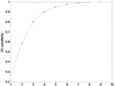
Fig. 2The curves of the C0C with different SNRs and r
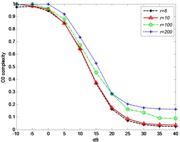
Table 1The summary of the selected parameter values
Complexity | Parameters | Value |
ApEn | Embedding dimension Tolerance Delay time | 2 0.2 std 1 |
SampEn | Embedding dimension Tolerance Delay time | 2 0.2 std 1 |
FuzzyEn | Embedding dimension Tolerance Parameter Delay time | 2 0.2 std 2 1 |
PermEn | Embedding dimension Delay time | 6 1 |
LZC | Parameter | median value |
Parameter | 10 |
From the procedures of the sevens, we can see that ApEn derives from correlation dimension. They have many similarities in their forms and calculation. SampEn and FuzzyEn are two modifications of ApEn in different aspects. Although, PermEn have somewhat similar in form to ApEn, e.g. phase-space reconstruction, but it calculates complexity in ShEn form. Thus, we can classify the complexities into two categories: one is the ApEn, SampEn and FuzzyEn, the other is PermEn and ShEn. As to the rest of the sevens, LZC and , we put them into another category, for they have threshold parameters for coarse-graining or as the boundary of periodicity and randomness. To compare the performance of the sevens, we need to reduce the influence of parameters, so the communal parameters should be consistent. The setting of parameters is within the recommended values of their original references. It is suggested that the tolerance of ApEn, SampEn and FuzzyEn should be set 0.1-0.25 std. The embedding dimension is suggested to set as 2 or 3. We set them as 0.2 std and 2. Particularly, though PermEn has the phase-space reconstruction procedure which has the same form as ApEn, FuzzyEn and PermEn, it is essentially different. For PermEn, vectors come from the phase-space reconstruction are not to be compared. Comparisons exist within the vectors. For the other two, comparisons are implemented between vectors to calculate the distance. So, the embedding dimension of PermEn is different from the others. Large will extremely increase the calculation time, and we set .
3. Performance of complexities in simulation signals
3.1. Performance in sinusoidal signals with additive noise
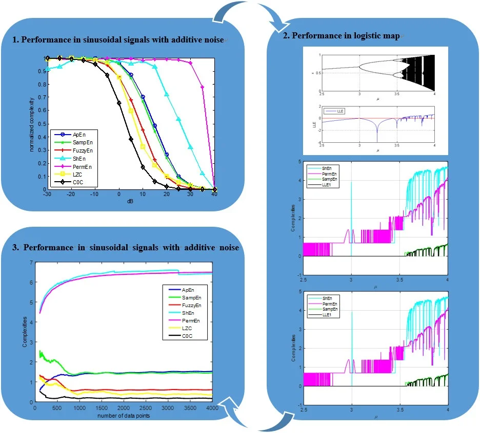
To figure out the performance of different complexities in rolling bearings, it is the primary and paramount to test in periodical signals with different intensity noise, where the sine wave is the simplest periodical signal. Now, we set a class of simulation signals defined as , where and represents the additive noise. The sampling frequency is 10000 Hz with 1 s duration. Fig. 3 shows the complexities with different SNRs. To be more vivid, all the complexities have been normalized.
Fig. 3The curve of seven complexities versus SNRs
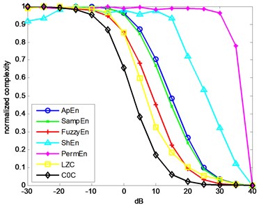
It is obvious to see that all the complexities tend to descend with the decreasing of the additive noise. The complexities should decrease with the decreasing of the additive noise. Among the sevens, ShEn and PermEn are the worst, since they do not have a good monotonous tendency. The rests of complexities present good monotonicity. Among them, ApEn the rightmost is the most sensitive to the noise, and the leftmost is the most insensitive to the noise.
3.2. Performance in logistic map
In Section 3.1, we have discussed the performance of seven complexities in a specific group of simulation signals. In this part, we will use more general simulation signals. The logistic map can be taken as an easy platform for it can generate periodical and chaotic signals. As many references shown, bearings are nonlinear components and many researches have reported nonlinear phenomena such as chaos, bifurcations and quasi-periodicity in bearings [38-40]. The logistic map is an easy nonlinear system, where it can be simple mathematical written as . Fig. 4 shows the process of the logistic map where , meanwhile, it shows the largest Lyapunov exponent (LLE) of the logistic map. Where means the system is periodical. means bifurcation occurs, and means chaotic behaviors occur. In the logistic map, the period 2 bifurcation happens at ; the 4 bifurcation happens at . After , there is a short period 3.
Analogically, we have calculated the seven complexities of the logistic map, and the results are shown in Fig. 5. The LLE is a reference of the sevens. The trend of the sevens should be similar to the LLE When . Let’s define a term of which satisfies that when , 0 when It is observed that PermEn has quite a few fluctuations before . ShEn has some platforms before . FuzzyEn has something wrong around and before . The reason of that must lie in the fuzzy membership of the FuzzyEn. LZC and have some wrong value about , where there exist chaotic behaviors, but both have values close to zero. All the sevens exhibit the short period 3 after . As it shows, ApEn and SampEn almost coincide with . In this part, ApEn and SampEn have the best performance. It should be notice that the application scope of the is narrow. It only can be calculated in the determined chaos systems. It cannot be computed with an arbitrary time series.
Fig. 5The seven complexities of the logistic map
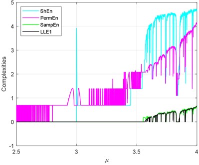
a) ShEn, PermEn and SampEn versus
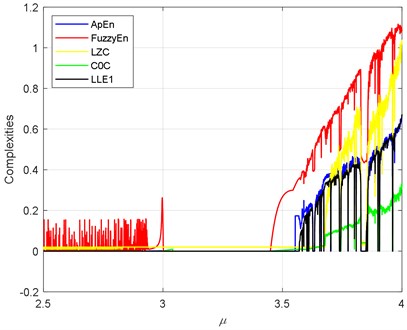
b) ApEn, FuzzyEn, LZC and versus
3.3. Performance in rate of convergence
The length of data can affect the complexities value too. By using the data where the complexities are not convergent is inaccurate. In this part, we will make certain the performance in rate of convergence of the seven complexities, and it is a supplementary performance of complexities. In order to study the influence of data length on the sevens, we use the simulation signal in Section 3.1 with SNR = –10 dB as an example. The length is from 100 to 4000, as illustrated in Fig. 6.
Fig. 6The curve of seven complexities versus SNRs
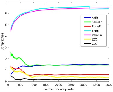
As we can see, PermEn and ShEn have similar increasing convergence trend, and the complexities value are convergent after 2000 data points. SampEn, FuzzyEn, LZC and have similar convergence trend. The complexities valued have a fluctuant decreasing trend. ApEn is different from the above, and it has a fluctuant increasing trend. From the comparison of convergence rate, we can confirm that is the best for it can be convergent about 1000 data points. ShEn and PermEn are no doubt the worst. To be more accurate and explicable, the length of each data should beyond 2000.
3.4. Brief summary of comparisons of simulation signals
From the three comparisons of simulation signals above, we can have some brief conclusions. Primarily, every complexity conforms to the basic principle i.e. the higher the regularity is, the lower the complexities value. Among them, the performances of ShEn and PermEn are dissatisfactory. Take ShEn as an example, the parameter of average filling of the histogram () must be set. Though, to be a certain extent, such a method can improve anti-noise performance, the complexity still has its inherent problems. For instance, it is relatively insensitive to the changes in the tails of the distribution and slow convergence. Similarly, LZC and have their inherent problems too. Coarse-graining may change the dynamic properties of the original time series. As to , it is lack of rigor to define a threshold as the boundary of periodicity and randomness. Relatively, ApEn and SampEn perform better than the others. As to a modification of ApEn, we consider that SampEn has the best performance among them. Thus, we will take SampEn as the benchmarking of the seven complexities.
4. Complexities comparisons in bearings’ run-to-failure data
In Section 3, we have used three methods to judge different aspects performance of the seven complexities in simulation signals. In this section, we will discuss the sevens in real signals i.e. the two bearings’ run-to-failure data. The failure form of the Example 1 is inner race fault, the other one is outer race fault.
4.1. Example 1 (inner race fault)
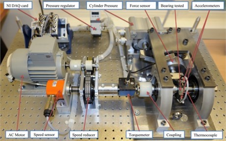
The Example 1 is from the IEEE PHM 2012 Prognostics Challenge data and the data were provided by FEMTO-ST Institute [41]. The purpose of the challenge was to estimate the remaining useful life of bearings. FEMTO-ST Institute has made an experimentation platform which is named PRONOSTIA as shown in Fig. 7. In this challenge, the data were monitored with 3 different loads. There were 6 complete run-to-failure data for training and 11 truncated data for predicting the remaining useful life. Tests were stopped when the vibration signal reached 20 g. However, we have no idea of the failure type of the bearings. In this paper, the first dataset is taken as the Example 1 within 2803 files. The parameters of the test and bearings are listed in Table 2.
Fig. 7Overview of PRONOSTIA
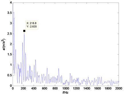
As a fact that we don’t know the failure type of the Example 1, we can study the envelop spectrum of it. The envelope spectrum of the last file of the Example 1 is shown in Fig. 8. By calculation of characteristics frequencies of the test, we can obtain the ball pass frequency on inner race is 221.66 Hz, the ball pass frequency on outer race is 168.34 Hz and fundamental train frequency is 12.95 Hz. In Fig. 8, there is a peak at 218.8 Hz. So, we can infer that the final failure type of Example 1 is inner race fault.
Table 2The parameters of the test and bearings.
Pitch diameter () | Number of rolling elements () | Bearing’s rolling element diameter () | Sample frequency () | Sample length () | Record frequency | Operating condition of Example 1 |
25.6 mm | 13 | 3.5 mm | 25.6 kHz | 25600 | 10s | 1800 rpm and 4000 N |
Fig. 8The envelope spectrum of e Example 1’s last file data
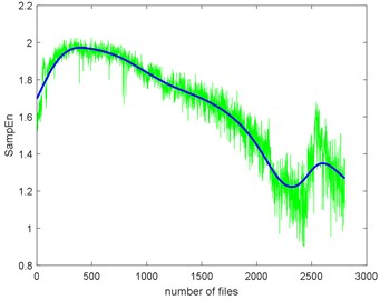
The seven complexities of the Example 1 are calculated as shown in Fig. 9. The seven complexities present a downtrend. They show consistent results, however, the ShEn seems to have more fluctuation. Among them, ApEn, SampEn and LZC seem to be more similar. Take SampEn as an example, before #500 (where # means the number file), the complexity increases to a peak and then decreases for a long time. As the figure shows, there is a local peak appeared about #2400 to #2600. Before #500, oil film is not fully formed is the reason of the arise of the complexities. When formed, the complexities’ decreasing indicate that the fault of the bearing is deepening. The reason for the peak around about #2400 to #2600 is probably the pitting of the surface are planished by the rotating. So, the signal may present not so periodical. And then, the new cracks appear making the signal more periodical, so the complexities are then dropped.
The complexities present a kind of similarity and can be explained with Fig. 3. Assume that the curves in Fig. 3 are seven functions (, ) that reflect monotonic decreasing, they have a similar trend. Take each file data as x () and put them to . If the functions are similar, then the results are similar too. To give quantitative similarity results, in this paper, we will propose a trend similarity index (TSI). Many similarity indexes are based on distance measures e.g. Manhattan distance, Euclidean distance, Kullback-Leibler divergence or correlation analysis e.g. Pearson correlation coefficient. Neither can measure the trend similarity of two sequences. In order to measure the trend of a time series, what comes to mind first is to analyze the derivatives. Certainly, we need to deburr the complexities curves. There we use the smoothing spline for fitting. Fig. 10 shows the SampEn deburred by smoothing spline with the smoothing parameter s equals to 1e-6, 1e-7 and 1e-8. As we can see, when 1e-6, the fitted SampEn exists a little fluctuation. When 1e-8, the smoothed SampEn doesn’t have a good fitting at the end of the data.
Fig. 9The seven complexities of Example 1
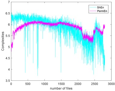
a) ShEn and PermEn
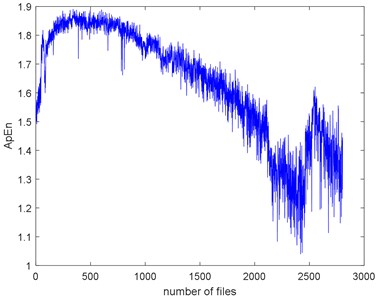
b) ApEn

c) SampEn
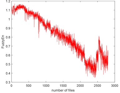
d) FuzzyEn
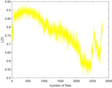
e) LZC
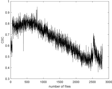
f)
To define the trend similarity of two same length time series, a direct way is to consider the derivatives of them. Fig. 11(a) shows three functions, where , , , we can consider that they have the same trend, for they have positive derivatives. Fig. 11b) shows two functions, where , . We can deem that where , they have the same trend, where , they have the different trend. By defining the ratio of the same trend length to the entire length, we can obtain the TSI, where the TSI of and is 50 %. In Section 3, we have concluded that SampEn present the best performance of the seven complexities in simulation signals, and then, we can have each TSI based on the SampEn deburred by smoothing spline which is shown in Table 3. From the results, we can clearly find that ApEn have extremely high similarity. ShEn and PermEn have relatively low similarity to the SampEn. Though, fitting parameters can affect the results of TSI, it is not an obstacle to estimate which complexity has higher similarity to SampEn.
Fig. 10The SampEn of Example 1 deburred by smoothing spline with the three smoothing parameters
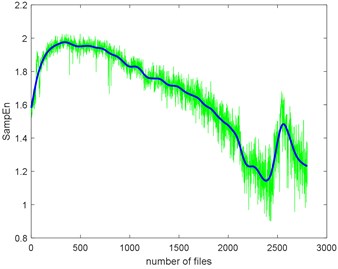
a) The smoothing parameter equals to 1e-6
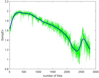
b) The smoothing parameter equals to 1e-7
c) The smoothing parameter equals to 1e-8
Fig. 11The example of trend similarity
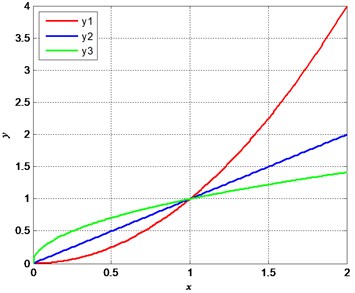
a), and
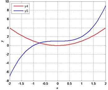
b) and
Table 3The TSI of each complexity based on the SampEn denoised by smoothing spline with different smoothing parameters
Complexity | TSI (1e-6) | TSI (1e-7) | TSI (1e-8) |
ApEn | 98.39 % | 99.50 % | 98.64 % |
FuzzyEn | 91.75 % | 97.25 % | 93.54 % |
ShEn | 82.22 % | 86.68 % | 89.75 % |
PermEn | 71.87 % | 69.44 % | 69.69 % |
LZC | 85.58 % | 91.75 % | 91.57 % |
85.26 % | 91.86 % | 93.72 % |
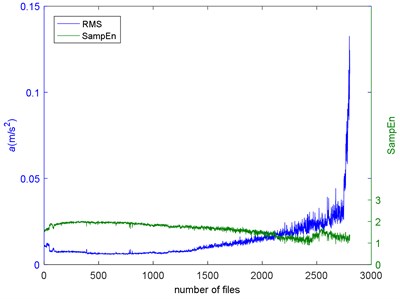
Intuitively speaking, the directly way to reflect the degradation of impact is the amplitude of defect frequency (ADF). The peaks at the envelope spectrum of impact of the Example 1 are calculated and make up the ADF as shown in Fig. 12. As we can see, there is a little fluctuation before #2750, and then there is a quick increasing. Accurately, the ADF measures the energy of the impact. It is a portion of the whole energy of the vibration signals. The root mean square (RMS) is a commonly used feature to measure the holistic energy of the signals. The RMS of the Example 1 is shown in Fig. 13 with SampEn. The increasing of RMS indicates the deepening of the deterioration. We can see that there is an opposite trend between the RMS and SampEn. When there is a pitting occurs on the rubbing surface, it will make energy concentration and the signal more periodical. So, the complexities go down. However, at the end of failure, the RMS increases quickly, but there is no sudden decreasing of SampEn. That’s can be explained when the bearing is closing to failure, there are more pitting on the rubbing surface, each pitting can cause the periodical signal, but the combined signal is not as periodical as the one caused by a pitting. So, the RMS and SampEn measure different properties of the signal.
Fig. 12The Example 1’s ADF
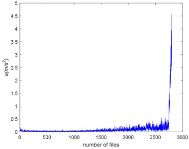
Fig. 13The RMS and SampEn of the Example 1
4.2. Example 2 (outer race fault)
Another run-to-failure data is used to verify the performance of the seven complexities. The data comes from the Intelligent Maintenance System (IMS) center [42]. The test rig is mounted four bearings on a shaft as shown in Fig. 14. In the test, four double row bearings typed Rexnord ZA-2115 were installed on the shaft. An accelerometer was installed on the test rig to monitor the vibration signal of the bearings. The parameters of the test and bearings are shown in Table 4. The bearing 2-1 which is the first bearing of the Set No. 2 is used as the Example 2. The failure type of the Example 2 is outer race defect which is shown in Fig. 15. The Example 2 has 982 files.
Table 4The parameters of the test and bearings.
Pitch diameter () | Number of rolling elements () | Bearing’s rolling element diameter () | Sample frequency () | Sample length () | Record frequency | Operating condition of Example 1 |
0.331 inches | 16 | 2.815 inches | 20 kHz | 20480 | 10 min | 2000 rpm and 6000 lbs |
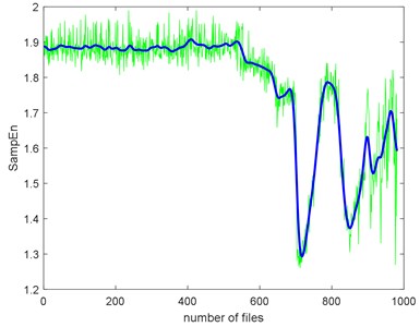
The complexities of Example 2 are shown in Fig. 16. We can see there is a similar trend. We use the SampEn as an example. Before #520, it presents stationary process and the bearing is in normal condition. We can see the complexity decreases linearly from #520 to #700 and the bearing is in slight defect condition. From #700 to #850, there is a peak and the condition is severe. From # 900 to the failure, the SampEn presents an increasing and the bearing is run to failure. On the whole, the SampEn is decreasing which is a same conclusion of Example 1. We can compare the RMS and ADF of the Example 2 to explore the reason why the trend of complexities is present like that.
Fig. 14The test rig of Example 2
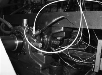
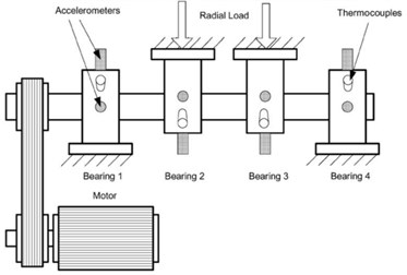
Fig. 15The failure type of Example 2
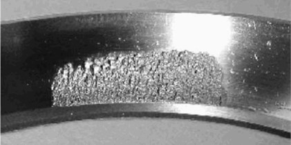
Fig. 16The seven complexities of Example 2
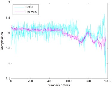
a) ShEn and PermEn
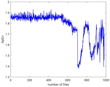
b) ApEn
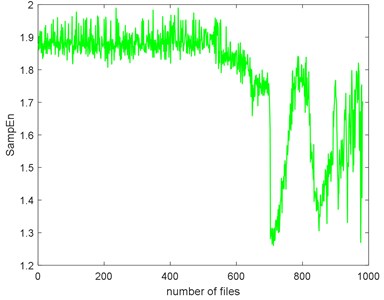
c) SampEn
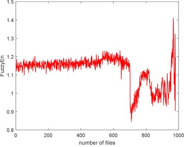
1
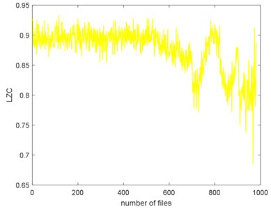
e) LZC
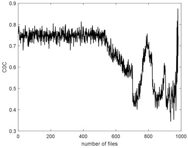
f)
Fig. 17 and Fig. 18 show the RMS and ADF of the Example 2. The trend of RMS and ADF is similar. Before #520, the RMS presents stationary and it increases linearly to #700. Between #700 and #850, the RMS experiences decreasing and then increasing. This is so-called “healing” phenomenon and have been stated detail in Ref. [7, 43, 44]. Form #900 to the end, the environment of the bearing is becoming violent. The RMS rises quickly to the failure.
Take SampEn as a baseline, we can have the TSI of each complexity too, as shown in Table 5. Before calculating TSI, the SampEn must be deburred. Fig. 19 shows the SampEn deburred by smoothing spline with the smoothing parameter s equals to 1e-3, 1e-4 and 1e-5. From the results, we can still find that ApEn has extremely high similarity to SampEn.
Fig. 17The Example 2’s RMS
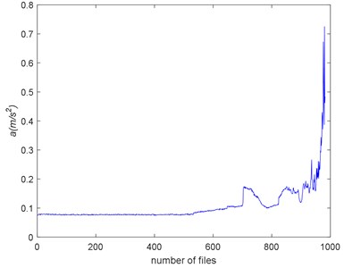
Fig. 18The Example 2’s ADF
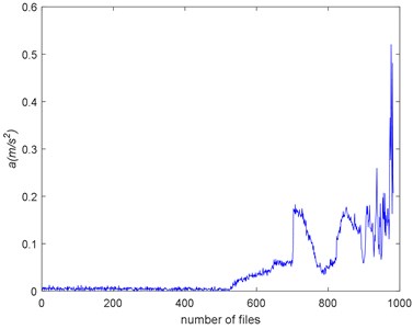
Fig. 19The SampEn of Example 2 deburred by smoothing spline with the three smoothing parameters
a) The smoothing parameter equals to 1e-3

b) The smoothing parameter equals to 1e-4
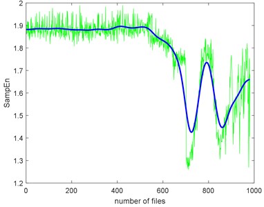
c) The smoothing parameter equals to 1e-5
Table 5The TSI of each complexity based on the SampEn denoised by smoothing spline with different smoothing parameters
Complexity | TSI (1e-3) | TSI (1e-4) | TSI (1e-5) |
ApEn | 89.69 % | 92.76 % | 90.92 % |
FuzzyEn | 69.59 % | 74.39 % | 69.59 % |
ShEn | 60.20 % | 61.94 % | 57.45 % |
PermEn | 64.80 % | 70.82 % | 63.67 % |
LZC | 67.14 % | 69.90 % | 67.86 % |
61.63 % | 55.92 % | 59.39 % |
5. Discussion
At present, we have completed the comparisons of the seven complexities. It can be seen that complexity is a reliable, robust feature of rolling bearings’ degradation. It can reflect the process stage of degradation. From the Example 1, we can move forward to see the ADF and RMS curves. The ADF shows a long time with nearly no significant characters until failure. That is universal phenomenon of inner race fault. The RMS seems to be better than ADF, it shows a slightly increasing until failure. We have plotted the RMS curves of the seventeen individuals of the IEEE PHM 2012 Prognostics Challenge data. Most of them manifest an increasing trend, but some of the others have no regularity. However, for complexity feature, it is destined to have a decreasing trend. With the deepening of the process, there must be defect occurs, whatever the type is. What will make a defect frequency, leading to the decreasing of randomness. In addition, there are many defect types, a punctate one can trigger characteristic frequency, hardly for a flaky one. In Ref. [17-19], Yan et al. have the similar conclusions that with the time elapses, the complexities are increasing. By carefully studying the references, we found that the key reason is about the experiment. Yan et al. did the experiment by cut a slot beforehand, thus making the process extremely changed.
In the paper, we have proposed an index of trend similarity. From the charts of two run-to-failure data, we can find this similarity. However, how to define the “trend” of a time series still need to study. In our work, we have tried every fitting method of curve fitting toolbox in MATLAB, and find that smoothing spline have a good result. But, how to select the smoothing parameter s is still unsolved. Furthermore, by finding that complexities are a good family feature of rolling bearings’ degradation, this paper gives a direction for dimensionality reduction of multi-features. A kind of family feature can be represented by a good one of it, thus can reduce dimensions in an initiative way.
6. Conclusions
In this paper, we have discussed and compared seven commonly used randomness complexities in simulation signals and real signals. By comparisons, we have found the similarity of complexities and explained it. In addition, we have defined a trend similarity index to measure the similarity of different complexities in run-to-failure bearings’ data. Finally, we can conclude that randomness complexity is a family feature of rolling bearings’ degradation. The complexities are similar, among the sevens, SampEn have the best performance, it can be a representative to represent the family feature of complexities.
References
-
Zhang B., Georgoulas G., Orchard M., Saxena A. Rolling element bearing feature extraction and anomaly detection based on vibration monitoring. Mediterranean Conference on Control and Automation, 2008, p. 1792-1797.
-
Boškoski P., Gašperin M., Petelin D., Juričić Đ. Bearing fault prognostics using Rényi entropy based features and gaussian process models. Mechanical Systems and Signal Processing, Vol. 52, Issue 53, 2015, p. 327-337.
-
Liao Z., Song L., Chen P., Zuo S. An automatic filtering method based on an improved genetic algorithm – with application to rolling bearing fault signal extraction. IEEE Sensors Journal, Vol. 17, 2017, p. 6340-6349.
-
Zhang B., Sconyers C., Byington C., Patrick R., Orchard M. E., Vachtsevanos G. A probabilistic fault detection approach: application to bearing fault detection. IEEE Transactions on Industrial Electronics, Vol. 58, 2011, p. 2011-2018.
-
Wang Y., Xiang J., Markert R., Liang M. Spectral kurtosis for fault detection, diagnosis and prognostics of rotating machines: a review with applications. Mechanical Systems and Signal Processing, Vol. 66-67, 2016, p. 679-698.
-
Randall R. B., Antoni J. Rolling element bearing diagnostics – a tutorial. Mechanical Systems and Signal Processing, Vol. 25, 2011, p. 485-520.
-
El Thalji I., Jantunen E. A summary of fault modelling and predictive health monitoring of rolling element bearings. Mechanical Systems and Signal Processing, Vol. 60, Issue 61, 2015, p. 252-272.
-
Jardine A. K. S., Lin D., Banjevic D. A review on machinery diagnostics and prognostics implementing condition-based maintenance. Mechanical Systems and Signal Processing, Vol. 20, 2006, p. 1483-1510.
-
Tandon N., Choudhury A. A review of vibration and acoustic measurement methods for the detection of defects in rolling element bearings. Tribology International, Vol. 32, 1999, p. 469-480.
-
Borghesani P., Pennacchi P., Chatterton S. The relationship between kurtosis- and envelope-based indexes for the diagnostic of rolling element bearings. Mechanical Systems and Signal Processing, Vol. 43, 2014, p. 25-43.
-
Rapp P. E., Schma T. Complexity measures in molecular psychiatry. Molecular Psychiatry, Vol. 1, 1996, p. 408-416.
-
Rapp P. E., Schmah T. I. Dynamical Analysis in Clinical Practice. Proceedings of the Workshop Chaos in Brain, 2000, p. 52-62.
-
Zhao S. F., Liang L., Xu G. H., Wang J., Zhang W. M. Quantitative diagnosis of a spall-like fault of a rolling element bearing by empirical mode decomposition and the approximate entropy method. Mechanical Systems and Signal Processing, Vol. 40, 2013, p. 154-177.
-
Yang Y., Yudejie, Cheng J. Roller bearing fault diagnosis method based on EMD energy entropy and ANN. Journal of Sound and Vibration, Vol. 294, 2006, p. 269-277.
-
Zheng J., Cheng J., Yang Y. A rolling bearing fault diagnosis approach based on LCD and fuzzy entropy. Mechanism and Machine Theory, Vol. 70, 2013, p. 441-453.
-
Pan Y. N., Chen J., Li X. L. Spectral entropy: a complementary index for rolling element bearing performance degradation assessment. Proceedings of the Institution of Mechanical Engineers, Part C: Journal of Mechanical Engineering Science, Vol. 223, 2009, p. 1223-1231.
-
Yan R., Gao R. X. Complexity as a measure for machine health evaluation. IEEE Transactions on Instrumentation and Measurement, Vol. 53, 2004, p. 1327-1334.
-
Yan R., Gao R. X. Approximate entropy as a diagnostic tool for machine health monitoring. Mechanical Systems and Signal Processing, Vol. 21, 2007, p. 824-839.
-
Yan R., Liu Y., Ga R. X. Permutation entropy: a nonlinear statistical measure for status characterization of rotary machines. Mechanical Systems and Signal Processing, Vol. 29, 2007, p. 474-484.
-
Javed K., Gouriveau R., Zerhouni N., Nectoux P. Enabling health monitoring approach based on vibration data for accurate prognostics. IEEE Transactions on Industrial Electronics, Vol. 62, 2014, p. 647-656.
-
Deng W., Zhang S., Zhao H., Yang X. A novel fault diagnosis method based on integrating empirical wavelet transform and fuzzy entropy for motor bearing. IEEE Access, Vol. 6, 2018, p. 35042-35056.
-
Zhao H., Sun M., Deng W., Yang X. A new feature extraction method based on EEMD and multi-scale fuzzy entropy for motor bearing. Entropy, Vol. 19, 2017, p. 1-14.
-
Li H., Wang Y., Wang B., Sun J., Li Y. The application of a general mathematical morphological particle as a novel indicator for the performance degradation assessment of a bearing. Mechanical Systems and Signal Processing, Vol. 82, 2017, p. 490-502.
-
Wang B., Hu X., Li H. Rolling bearing performance degradation condition recognition based on mathematical morphological fractal dimension and fuzzy C-means. Measurement, Vol. 109, 2017, p. 1-8.
-
Shannon C. E. A mathematical theory of communication. Bell System Technical Journal, Vol. 27, 1948, p. 3-55.
-
Renyi A. On Measures of Information and Entropy. Proceedings of the Fourth Berkeley Symposium on Mathematical Statistics and Probability, Vol. 1, 1978, p. 547-561.
-
Kolmogorov A. N. On tables of random numbers. Theoretical Computer Science, Vol. 207, 1963, p. 369-376.
-
Leung Yan Cheong S., Cover T. Some equivalences between Shannon entropy and Kolmogorov complexity. IEEE Transactions on Information Theory, Vol. 24, 1978, p. 331-338.
-
Lempel A., Ziv J. On the complexity of finite sequences. IEEE Transactions on Information Theory, Vol. 22, 1976, p. 75-81.
-
Pincus S. M. Approximate entropy as a measure of system complexity. Proceedings of the National Academy of Sciences of the United States of America, Vol. 88, 1991, p. 2297.
-
Richman J. S., Moorman J. R. Physiological time-series analysis using approximate entropy and sample entropy. American Journal of Physiology Heart and Circulatory Physiology, Vol. 278, 2000, p. H2039.
-
Costa M., Goldberger A. L., Peng C. K. Multiscale entropy analysis of biological signals. Physical Review E Statistical Nonlinear and Soft Matter Physics, Vol. 71, 2005, p. 021906.
-
Bandt C., Pompe B. Permutation entropy: a natural complexity measure for time series. Physical Review Letters, Vol. 88, 2002, p. 174102.
-
Chen W., Wang Z., Xie H., Yu W. Characterization of surface EMG signal based on fuzzy entropy. IEEE Transactions on Neural Systems and Rehabilitation Engineering, Vol. 15, 1998, p. 267-272.
-
Fang C., Fanji G. A new measurement of complexity for studying EEG mutual information. Acta Biophysica Sinica, Vol. 14, 1998, p. 508-512, (in Chinese).
-
Zhijie C., Jie S. Modified C0 complexity SND applications. Journal of Fudan University (Natural Science), Vol. 47, 2008, p. 791-796.
-
Zhijie C., Jie S. Convergence of C0 complexity. International Journal of Bifurcation and Chaos, Vol. 19, 2011, p. 977-992.
-
Mevel B., Guyader J. L. Routes to chaos in ball bearings. Journal of Sound and Vibration, Vol. 162, 2007, p. 471-487.
-
Tiwari M., Gupta K., Prakash O. Effect of radial internal clearance of a ball bearing on the dynamics of a balanced horizontal rotor. Journal of Sound and Vibration, Vol. 238, 2000, p. 723-756.
-
Yuan W., Liu S. Numerical analysis of the dynamic behavior of a rotor-bearing-brush seal system with bristle interference. Journal of Mechanical Science and Technology, Vol. 33, Issue 8, 2019, p. 3895-3903.
-
Nectoux P., Gouriveau R., Medjaher K., Ramasso E., Morello B., Zerhouni N., et al. Pronostia: an experimental platform for bearings accelerated life test. IEEE International Conference on Prognostics and Health Management, Denver, USA, 2012.
-
Qiu H., Lee J., Lin J., Yu G. Wavelet filter-based weak signature detection method and its application on rolling element bearing prognostics. Journal of Sound and Vibration, Vol. 289, 2006, p. 1066-1090.
-
Williams T., Ribadeneira X., Billington S., Kurfess T. Rolling element bearing diagnostics in run-to-failure lifetime testing. Mechanical Systems and Signal Processing, Vol. 15, 2001, p. 979-993.
-
El Thalji I., Jantunen E. A descriptive model of wear evolution in rolling bearings. Engineering Failure Analysis, Vol. 45, 2014, p. 204-224.
Cited by
About this article

We like to acknowledge the support from the National Natural Science Foundation of China (Grant No. 51541506). We also appreciate the IEEE Reliability Society and FEMTO-ST Institute and the Centre for Intelligent Maintenance System, University of Cincinnati for providing the experimental data.
