Abstract
To reduce the adverse effects of the ice on aerodynamic characteristics, a new NREL Phase VI wind turbine blade which is suitable to rime ice environments is developed through the blunt trailing-edge optimization. The parametric control equations of blunt trailing-edge airfoil are established by adopting the airfoil profile integration theory and B-spline curve, and the curve fitting of the airfoil’s rime ice from LEWICE software is carried out using the linear interpolation algorithm with equidistant and equiangular step lengths. The S809 airfoil under rime ice conditions is optimized to maximize the lift coefficient by the particle swarm optimization (PSO) coupled with GAMBIT and FLUENT, and a NREL Phase VI blade is formed with the optimized airfoil S809-BT (with BT the blunt trailing-edge). The blade’s rime ice is obtained through using the polynomial fitting to deal with projection point coordinates of airfoils’ ice shapes in lagging and flapping surfaces, and the pressure coefficient, flow characteristics, torque and output power of icy sharp and blunt trailing-edge blades are investigated. The results indicate that in rime ice conditions, compared with those of sharp trailing-edge blade, the pressure difference and vortex size of blunt trailing-edge blade become larger, and the torque and output power increase by 4.36 %, 1.55 % and 2.88 % at 7 m/s, 15 m/s and 20 m/s, respectively. The research provides significant guidance for improving the aerodynamic performance of wind turbine blade considering the icing effects.
1. Introduction
The wind energy resources are mainly concentrated in the contraction zones of coast and open continent. Owing to the cold climate in these regions, the ice often occurs on the wind turbine blade. The icing decreases the aerodynamic performance, wind energy utilization, and annual power generation [1-6], and increases the static and dynamic loads, and vibrational frequency [7, 8]. It is necessary to study a reasonable and effective method to improve the aerodynamic and structural characteristics of icy blades.
The airfoil, that is, the cross-section of the blade, directly affects the performance. The blunt trailing-edge modification and direct optimization can improve the aerodynamic characteristics, structural strength and stiffness of rough airfoils. Baker et al.[9] investigated the airfoils with symmetrical trailing-edge thickness through experiments, and found that the lift-drag ratio improved and the sensitivity to leading-edge roughness reduced by increasing appropriate trailing-edge thickness. Yang et al. [10] used the Computational fluid dynamics (CFD) method to study the aerodynamic performance of blunt trailing-edge airfoil, and the results showed that the maximum lift coefficient increased and the effects of the leading-edge roughness on lift characteristics decreased. Zhang et al. [11, 12] numerically studied the effects of the blunt trailing-edge modification on the aerodynamic performance enhancement of the airfoil with sensitive roughness height and position.
Miller et al. [13] performed the multi-objective aero-structural optimization of thick flatback airfoils using a genetic algorithm, and found that the obtained airfoils displayed a relative insensitivity to roughness. Chen et al. [14] presented an optimization method of wind turbine airfoil to improve the aerodynamic performance under typical rime ice conditions. Zhang et al. [15] carried out the optimization design of blunt trailing-edge airfoil by PSO coupled with XFOIL, then added a lug boss to obtain the rough airfoil, and numerically analyzed the lift-drag ratios, pressure coefficients and flow characteristics.
The above studies separately analyzed the effects of the blunt trailing-edge modification and direct optimization on aerodynamic characteristics of rough airfoils. In view of the advantages of two methods, this paper carries out the optimization design of blunt trailing-edge airfoil under rime ice conditions and investigates its impact on the aerodynamic performance enhancement of icy blades. Section 2 establishes the control equations of blunt trailing-edge airfoil profile, fits the airfoil’s rime ice obtained by LEWICE software, and optimizes the blunt trailing-edge airfoil with rime ice. Section 3 uses the optimized airfoil as the cross-sections from 46.6 % (with the radius of wind wheel) to 75 % to construct the NREL Phase VI blade, and applies the polynomial fitting to deal with projection point coordinates of airfoil’s ice shape in lagging and flapping surfaces. Section 4 studies the aerodynamic characteristics of sharp and blunt trailing-edge blades before and after icing.
2. Optimization design of airfoil under rime ice conditions
2.1. Expression method of blunt trailing-edge airfoil profile
The coordinates of blunt trailing-edge airfoil profiles before 0.4 (with the chord length) on the upper surface and 0.5 on the lower surface are given by the profile integration theory:
where and are the abscissa and longitudinal coordinates of the airfoil, is a quarter of the chord length, and is the shape function. , 1, 2, 3,…, in which is the argument, , , ,…, are the coefficients, and .
The coordinates after 0.4 on the upper surface and 0.5 on the lower surface are given by the B-spline curve:
where 1 and 2 represents the upper and lower profiles, and is relative position of the curve.
The last points formed by the profile integration theory, and the blunt trailing-edge points and , go through and , respectively, where and are the trailing-edge thickness and the ratio of trailing-edge thickness of upper surface to that of airfoil. So and are calculated by the Eqs. (2), and Eq. (3) is obtained:
2.2. Fitting of airfoil’s rime ice
The quantity and location of airfoil’s ice shape feature points vary with the airfoil type, chord length, and icing conditions. The linear interpolation algorithm in the first and fourth quadrants with equidistant step length and the second and third quadrants with equiangular step length is used to fit the rime ice so as to remain the number of feature points unchanged and realize the automatical mesh partition in the optimization. The coordinate formulas of interpolation points using the equal angle as the step length are as follows:
where and are the coordinates of rime ice feature points before the interpolation, are the coordinates of points obtained after the interpolation, is the -th key point of rime ice shape, and is the angle between the axis and connection line of the interpolation point and coordinate origin.
2.3. Optimization design
PSO coupled with GAMBIT and FLUENT is applied to optimize the blunt trailing-edge airfoil under rime ice conditions. The .jou file realizes the parameterized geometric modeling, computational domain establishment and mesh generation in GAMBIT, and the automatic computation in FLUENT.
The second to twelfth coefficients of shape function [16], the blunt trailing-edge thickness and its distribution ratio, and the B-spline control parameters are selected as design variables:
In order to ensure that the profile has the airfoil’s shape characteristics, the boundary constraints of optimization variables are:
Moreover, the lift coefficient of optimized blunt trailing-edge airfoil should be higher than that of sharp trailing-edge airfoil :
The lift coefficient is a significant index to measure the aerodynamic performance of wind turbine airfoil [17]. So the design objective is to maximize the lift coefficient:
2.4. Optimization example
The optimal design is performed for S809 airfoil with the relative thickness of 21 % at 0.395 and relative camber of 0.99 % at 0.823. According to Ref. [17], the icing parameters are given in Table 1 and is 0.267 m.
Table 1Rime ice conditions
Icing parameters | Air speed () / (m/s) | Angle of attack () / (°) | Atmospheric pressure () / Pa | Liquid water content (LWC) / (g/m3) | Water droplet diameter (MVD) / (μm) | Ambient temperature () / (°C) | Ice accretion time () / s |
Value | 50 | 2 | 101330 | 0.08 | 20 | –7 | 1800 |
The .jou file in GAMBIT is compiled to automatically establish the computational domain and generate the grid, and the results are stored in the .msh file. The computational domain consists of a semicircle with a diameter of 30 and a rectangle of size 30×20, and is divided into quadrilateral surfaces ANIH, NMJI, MLKJ, LFGK, FEDG, DCHG and CBAH, as shown in Fig. 1. The chord line of the airfoil is horizontal, and its end coincides with the center of the semicircle. The division method of each edge is given in Table 2, and the seven surfaces are discretized by the C-type structured grid, as shown in Fig. 2. The first boundary layer height is 0.000010512, and 1. The 200 nodes are arranged on the airfoil with rime ice, and the overall grids consist of 13520 quadrilateral and 13832 nodes. The edges BA, ANMLF and FE are defined as the velocity inlet, and the inlet velocity direction is from left to right. The pressure outlet is applied for BC, CD and DE, and the atmospheric pressure is zero. The edges HIJKG and GH are set to be no-slip and static wall boundary conditions.
Fig. 1Computational domain of airfoil
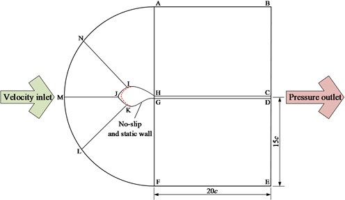
Table 2Division of edges of airfoil’s computational domain
Edges | Specified conditions | Mesh law |
AN, NM, ML, LF | Division direction, interval count, continuity ratio | Bi-exponent |
BC, AH, NI, MJ, LK, FG, ED, HI, IJ, JK, KG | Division direction, interval count, division lengths at the start and end of the edge | First length |
HG, CD | Division direction, interval count, continuity ratio | Successive ratio |
AB, HC, GD, FE | Division direction, interval count, division lengths at the start of the edge | First length |
The .jou file calls the .msh file to initialize and calculate the flow field while saving the results of lift and drag coefficients. The SST - turbulence model suitable to the wake flow of blunt trailing-edge airfoil is chosen to close the governing equations. The second-order upwind difference scheme is adopted for the discretization of each equation. The SIMPLE algorithm is used to solve the pressure and velocity coupling equation. The convergence criteria of continuity component, velocity component, and are all 10-4.
Fig. 2Grids of icy airfoil
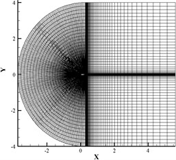
a) Global grids
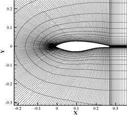
b) Local grids
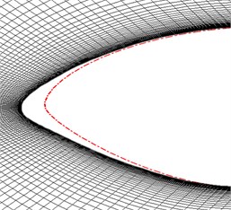
c) Grids near the leading-edge
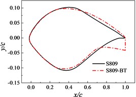
The initial optimization conditions are as follows: the Reynolds number Re is 106, the lift coefficient of S809 airfoil with rime ice is 0.3133 which is in close agreement with the result of Ref. [18], the sizes of population and dimension of variables are both 20, the learning factors and are both 2, the inertia weight is given by , is the current iteration number, the maximum iteration number is 300, the maximum inertia weight is 0.9, and the minimum inertia weight is 0.4. The S809-BT airfoil with the trailing-edge thickness of 0.0445 and thickness distribution ratio of 1:13.35 is obtained, as shown in Fig. 3.
Fig. 3S809 and S809-BT airfoils
3. Aerodynamic performance calculation method of blades with rime ice
3.1. Sharp trailing-edge blade
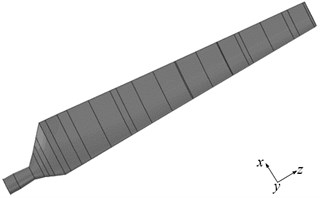
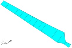
The NREL Phase VI wind turbine has two blades which use the S809 airfoil from the 25 % radial section to blade tip. The radius of wind wheel is 5.029 m, and the pitch angle of blade tip is 3°. The cut-in wind speed is 5 m/s, the rated power is 19.8 kW, and the rotational speed is 71.63RPM. The airfoil’s aerodynamic center is selected as the torsion center. According to the linear distributions of chord length and torsion angle along the span-wise direction in Ref. [19], the conversion formulas of space coordinates of each cross-section are as follows, and the three-dimensional model is shown in Fig. 4:
where and is two-dimensional coordinates of the -th point on each cross-section before the transformation, is span-wise coordinate of the -th cross-section,, , is three-dimensional coordinates of the -th point on the -th cross-section after the transformation, and and are chord length and torsion angle of the -th cross-section, respectively.
Fig. 4Three-dimensional model of sharp trailing-edge blade
3.2. Sharp and blunt trailing-edge blades with rime ice
The rime ices of multiple cross-sections are obtained from LEWICE and processed by the linear interpolation algorithm. The feature point coordinates of ice shapes of adjacent sections are mapped into lagging and flapping surfaces, and the space curves of rime ices on the blade surface are formed by using the polynomial fitting deal with projection points.
The blade with the length of is divided into segments along the -axis, and key points are gained after fitting the airfoil’s rime ice. So the ice shape space curves along the span-wise direction form, which have discrete points of group, and the polynomial fitting formulas are as follows:
where , , are coordinates of the -th point on the -th space curve along the chord-wise, perpendicular to chord-wise and span-wise directions, respectively, and , , ,…, are polynomial fitting parameters. Fig. 5 gives two NREL Phase VI blades with S809 airfoil between 25 % radial section to blade tip and optimized S809-BT airfoil between 46.6 % and 75 % radial sections after icing, respectively.
Fig. 5Sharp and blunt trailing-edge blades with rime ice (Blue represents rime ice)
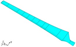
a) Icy sharp trailing-edge blade
b) Part of icy sharp trailing-edge blade
c) Icy blunt trailing-edge blade
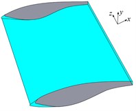
d) Part of icy blunt trailing-edge blade
3.3. Computational domain of blade
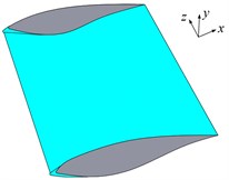
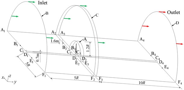
Only half of the flow field is analyzed because the wind wheel rotates periodically around the -axis. The blade’s computational domain is a semi-cylindrical body and divided into three static outer domains B, C, D, and one rotating inner domain A, as shown in Fig. 6. The blade is located in the center of domain A, and the blade root is 0.508 m away from the wheel center.
Fig. 6Computational domain of blade
3.4. Grid generation of blade
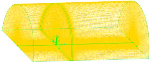
The division method of edges and arcs of blade’s computational domain is given in Table 3. The structured and unstructured quadrilateral grids are used to divide the surface, top and bottom of the blade. The inner and outer domains are divided by unstructured and hexahedral structured grids, respectively. For C domain, the division in the order of the edge, surface and volume is carried out to obtain hexahedral structured grids. The common surfaces between B domain and A domain and between B domain and C domain are defined as mapping source surfaces to establish the volume mesh of B domain, and the same mesh method is applied in D domain. About 4 million grids are generated, as shown in Fig. 7, and is less than 2.
Table 3Division of edges and arcs of blade’s computational domain
Edges or arcs | Specified conditions | Mesh law |
D1E1, C1B1, D2E2, C2B2, D3E3, C3B3, D4E4, C4B4 | Division direction, interval count, division lengths at the start and end of the edge | First length |
A1F1, A2F2, A3F3, A4F4, B2E2, B3E3, C1D1, C2D2, C3D3, C4D4 | Division direction, interval count, continuity ratio | Successive ratio |
A1A2, A2A3, A3A4, B2B3, C1C2, C2C3, C3C4, D1D2, D2D3, D3D4, F1F2, F2F3, F3F4, E2E3, A1B1, A2B2, A3B3, A4B4, E1F1, E2F2, E3F3, E4F4 | Division direction, interval count, division lengths at the start of the edge | First length |
Fig. 7Grid of icy blade
3.5. Boundary conditions and solving control parameters
The faces A1B1C1D1E1F1, A1A2F2F1, A2A3F3F2 and A3A4F4F3 are velocity inlet boundaries, and the face A4B4C4D4E4F4 is a pressure outlet boundary. The face B2B3E3E2 is the interface between stationary and rotating domains, and is set as the interior. The bottom of semi-cylindrical body is set as periodic boundary, and the blade surface is set as static and non-slip wall. The MRF method and SST - model are selected. Based on the pressure solver, the governing equation is solved by the SIMPLE algorithm. The pressure-velocity coupling treatment uses the PRESTO! format. The second-order upwind style is adopted for other discrete schemes. The convergence criteria of all variables are less than 10-5.
4. Results and analysis
4.1. Pressure coefficient
Fig. 8(a) and 8(b) show that after the sharp trailing-edge blade is covered with rime ice, the pressure coefficient and the area enclosed by the pressure curve are almost unchanged, except for the pressure coefficients on the suction surfaces of 95 % radial section at 7 m/s and 57 % radial section at 10 m/s. The pressure coefficient on the suction surface increases for –0.12~0 m and 0.075~0.26 m of 95 % radial section at 7 m/s and –0.12~0.05 m of 57 % radial section at 10 m/s, and is basically unchanged elsewhere. The pressure curve area reduces a little, which shows that the lift coefficient decreases slightly. In Fig. 8(c), the pressure coefficients and curve areas at 25 % and 57 % radial sections are also unchanged at 15 m/s. For 30 %, 80 % and 95 % radial sections, the pressure coefficient on the pressure surface decreases and that on the suction surface increases at –0.2~–0.05 m, –0.14~0.24 m and –0.12~0.24 m, respectively, and so the curve area evidently decreases. The reason of these phenomena is that the rime ice makes the blade surface be rough, which increases the flow disturbance.
Under rime ice conditions, compared with the sharp trailing-edge blade, the pressure coefficient on the pressure surface of blunt trailing-edge blade increases at 7 m/s, decreases at 10 m/s, and increases for –0.02~0.34 m at 15 m/s. The pressure coefficient on the suction surface decreases for –0.18~–0.08 m and 0.09~0.4 m at 7 m/s, –0.04~0.31 m and 0.37~0.4 m at 10 m/s, and is almost unchanged at 15 m/s. The pressure curve area evidently increases, and the aerodynamic performance improves. This is because that the blunt trailing-edge design reduces the sensitivity of the airfoil to leading-edge roughness, which decreases the flow disturbance induced by the rime ice.
4.2. Flow distribution
Fig. 9 shows when 7 m/s, there is no flow separation on each cross-section of sharp trailing-edge blade, and 25 % and 30 % radial sections of sharp trailing-edge blade with rime ice. Small separation vortexes occur on the trailing-edge of suction surface at 57 %, 80 % and 95 % radial sections for icy blade, and are similar in size. When 10 m/s, a vortex starts to occur on the trailing-edge of suction surface at 57 %, 80 % and 95 % radial sections, and its size increases first and then decreases as the cross-section approaches the blade tip before and after icing. The size of vortices at 57 % and 95 % radial sections increases after icing, but basically remains unchanged at the 80 % radial section. When 15 m/s, there exists a vortex on the trailing-edge of suction surface at the 25 % radial section, and a pair of vortices with opposite direction of rotation and large differences in size exists on the suction surface at 30 %, 57 % and 95 % radial sections before and after icing. At the 80 % radial section, the vortex on the suction surface has shed and begun to reform before icing, but after icing, a pair of vortices with opposite rotation direction and large differences in size has newly formed. That is to say, the vortex on the suction surface increases until it sheds and then reforms and gradually increases as the section approaches the blade tip, and the vortex starts shedding in advance after icing.
For the blunt trailing-edge blade with rime ice, the flow separation has occurred on the trailing-edge of suction surface, but the vortex has not yet formed at 7 m/s. A pair of vortices which rotate in opposite directions and have large differences in size occurs on the trailing-edge of suction surface at 10 m/s and 15 m/s, and is larger than that on the sharp trailing-edge blade.
Fig. 8Pressure coefficients at different cross-sections before and after icing
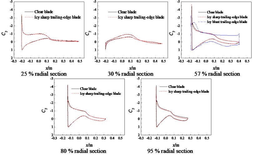
a)7 m/s
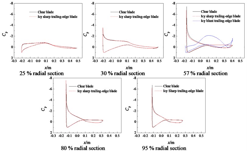
b)10 m/s
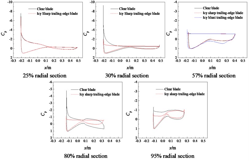
c) 15 m/s
Fig. 9Flow distribution at different cross-sections before and after icing
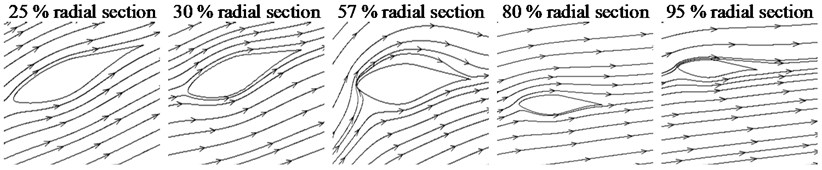
a) Sharp trailing-edge blade (7 m/s)
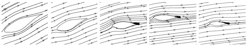
b) Icy sharp trailing-edge blade (7 m/s)
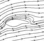
c) Icy blunt trailing-edge blade ( 7 m/s)
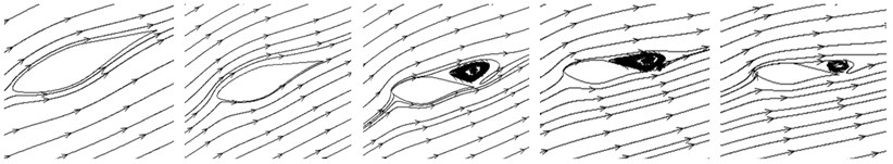
d) Sharp trailing-edge blade (10 m/s)
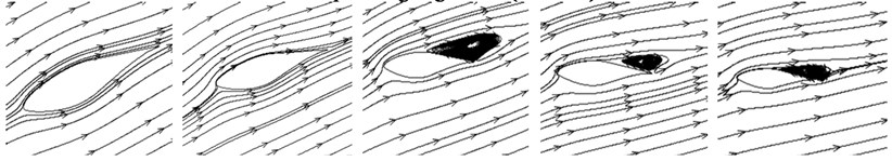
e) Icy sharp trailing-edge blade (10 m/s)
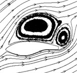
f) Icy blunt trailing-edge blade (10 m/s)
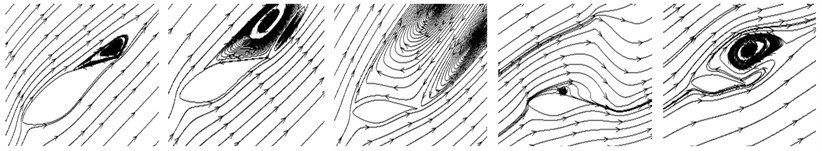
g) Sharp trailing-edge blade (15 m/s)
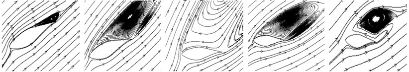
h) Icy sharp trailing-edge blade (15 m/s)
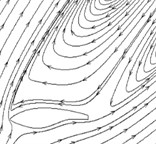
i) Icy blunt trailing-edge blade (15 m/s)
4.3. Torque and output power
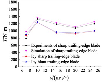
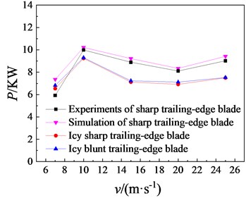
Fig. 10 shows for the torque and output power of sharp trailing-edge blade, the numerical results are slightly larger than experimental data form Ref. [20] due to neglect the effects of support structure and aero-elasticity, and they have similar variance tendency. and quickly increase first, then decrease gradually and increase slowly with the increase of wind speed for sharp and blunt trailing-edge blades before and after icing. and reduce obviously after icing, and the largest decline is 22.78 % at 15 m/s for two parameters which have the same rate of change according to . Compared with those of sharp trailing-edge blade under rime ice conditions, and of blunt trailing-edge blade increase by 4.36 %, 0.60 %, 1.55 %, 2.88 % and 0.40 % at 7 m/s, 10 m/s, 15 m/s, 20 m/s and 25 m/s, respectively. Overall, the icing makes and decrease, but the effect of icing can be reduced through the blunt trailing-edge optimization.
Fig. 10T and P of sharp and blunt trailing-edge blades with rime ice
a)
b)
5. Conclusions
The present work firstly performs the blunt trailing-edge optimization of S809 airfoil under rime ice conditions, and then the effects of the rime ice on the pressure coefficient, flow distribution, torque and output power of sharp and blunt trailing-edge NREL Phase VI blades are investigated. The main conclusions are as follows:
1) After the sharp trailing-edge blade is covered with rime ice, the pressure difference between upper and lower surfaces decreases at 95 % (7 m/s), 57 % (10 m/s) and 30 %, 80 %, 95 % (15 m/s) radial sections, respectively, and is unchanged at other cross-sections. The flow separation is more obvious, the size of vortices on the trailing-edge increases, and the vortices move toward the leading-edge. and reduce largely, and the biggest decrease is 22.78 % at 15 m/s.
2) The blunt trailing-edge optimization makes the pressure difference on the blade surface and the size of vortices larger than those of sharp trailing-edge blade under rime ice conditions. Therefore, and both increase by 4.36 %, 1.55 % and 2.88 % at 7 m/s, 15 m/s and 20 m/s, respectively, and change little for other wind speeds.
References
-
Han W., Kim J., Kim B. Study on correlation between wind turbine performance and ice accretion along a blade tip airfoil using CFD. Journal of Renewable and Sustainable Energy, Vol. 10, Issue 9, 2018, p. 023306.
-
Blasco P., Palacios J., Schmitz S. Effect of icing roughness on wind turbine power production. Wind Energy, Vol. 20, Issue 4, 2017, p. 601-617.
-
Alessandro Z., Michele D., Helmut K. Wind energy harnessing of the NREL 5MW reference wind turbine in icing conditions under different operational strategies. Renewable Energy, Vol. 115, 2018, p. 760-772.
-
Matthew C. H., Muhammad S. V., Tomas W., Nicklasson P. J., Sundsbø P. A. Effect of atmospheric temperature and droplet size variation on ice accretion of wind turbine blades. Journal of Wind Engineering and Industrial Aerodynamics, Vol. 98, Issue 12, 2010, p. 724-729.
-
Fortin G., Hochart C., Perron J. Wind turbine performance under icing conditions. Journal of Solar Energy Engineering, Vol. 11, Issue 4, 2008, p. 319-333.
-
Lee S., Hwang B., Kim T., Lee S. Aeroacoustic analysis of a wind turbine airfoil and blade on icing state condition. Journal of Renewable and Sustainable Energy, Vol. 6, Issue 4, 2014, p. 042003.
-
Tammelin B., Säntti K. Estimation of rime accretion at high altitudes – preliminary results. Proceedings of the BOREAS III, Saariselkä, Finland, 1996.
-
Huo F. P., Li Y. H., Chen Z. Y. Suggestions for improve wind turbine blade characteristics. Wind Engineering, Vol. 25, Issue 2, 2001, p. 105-114.
-
Baker J. P., Mayda E. A., Van Dam C. P. Experimental analysis of thick blunt trailing-edge wind turbine airfoils. Journal of Solar Energy Engineering, Vol. 128, Issue 4, 2006, p. 422-431.
-
Yang R., Li R. N., Zhang S. A., Li D. S. Computational analyses on aerodynamic characteristics of flatback wind turbine airfoils. Journal of Mechanical Engineering, Vol. 46, Issue 2, 2010, p. 106-110.
-
Zhang X., Wang G. G., Zhang M. J., Liu H. L., Li W. Numerical study of the aerodynamic performance of blunt trailing-edge airfoil considering the sensitive roughness height. International Journal of Hydrogen Energy, Vol. 42, Issue 29, 2017, p. 18252-18262.
-
Zhang X., Liu H. L., Wang G. G., Li W. Aerodynamic Performance of Blunt Trailing-edge Airfoil Considering Roughness Sensitivity Position. Transactions of the Chinese Society of Agricultural Engineering, Vol. 33, Issue 8, 2017, p. 82-89.
-
Miller M., Slew K. L., Matida E. The effect of aerodynamic evaluators on the multi-objective optimization of flatback airfoils. Conference on Science of Making Torque from Wind (TORQUE), Munich, Germany, 2016.
-
Chen J., Jiang C. H., Xie Y., Sun Z. Y., Wang H. Y. Optimization design of airfoil for wind turbine under typical rime icing conditions. Journal of Mechanical Engineering, Vol. 50, Issue 7, 2014, p. 154-160.
-
Zhang X., Wang G. G., Liu H. L., Li W. Study of optimization design method for asymmetric blunt trailing-edge airfoil of wind turbine. Journal of Engineering Thermophsics, Vol. 39, Issue 2, 2018, p. 326-334.
-
Jiang C. H. Aerodynamic Performance Analysis and Optimization Design of Wind Turbine with Iced Airfoil. Mechanical Engineering College, Chongqing University, China, 2014.
-
Han Y. Q., Palacios J., Schamitz S. Scaled ice accretion experiments on a rotating wind turbine blade. Journal of Wind Engineering and Industrial Aerodynamics, Vol. 109, 2012, p. 55-67.
-
Ren P. F., Xu Y., Song J. J., Xu J. Z. Numerical research on impact of icing on wind turbine blades. Journal of Engineering Thermophysics, Vol. 36, Issue 2, 2015, p. 313-317.
-
Hand M. M., Simms D. A., Fingersh L. J., Jager D. W., Cotrell J. R., Schreck S., Larwood S. M. Unsteady Aerodynamics Experiment Phase VI: Wind Tunnel Test Configurations and Available Data Campaigns. NREL Technical Report No. NREL/TP-500-29955, 2001.
-
Wang Y. F., Jiang Z., An Y. R. Turbulence model research based on numerical simulation of NREL PHASE VI wind turbine rotor. Chinese Journal of Hydrodynamics, Vol. 28, Issue 5, 2013, p. 606-614.
Cited by
About this article

This work was supported by the National Natural Science Foundation of China (Grant No. 51805369), the Natural Science Foundation of Tianjin (Grant No. 17JCYBJC20800), and the China Scholarship Council (Grant No. 201908120031 and 201908120062).
