Abstract
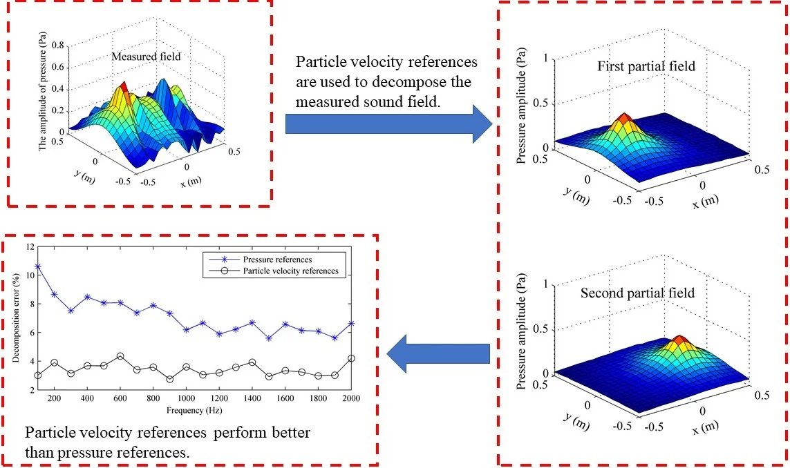
In existing partial field decomposition methods, the pressures are generally used as references. This paper is going to use the particle velocities as the references to decompose the sound field radiated by incoherent or partially coherent sources into mutually incoherent partial fields, and evaluate its performance by comparing with the method using pressure references. Both numerical simulations and experiment confirm the effectiveness of the method using particle velocity references for partial field decomposition and demonstrate its superiority over the method using pressure references, and it is also shown through numerical simulations that the particle velocity references almost always perform better than the pressure references as long as the references are located close to the sources and the directions of particle velocity references are perpendicular to the source plane as far as possible.
Highlights
- Particle velocity references are used to decomposes the incoherent sound field.
- Particle velocity references performs better than pressure references.
- Particle velocity references are less sensitive to position than pressure references.
1. Introduction
In order to accurately identify sound sources and visualize their associated sound fields via such technique as nearfield acoustic holography (NAH) [1-3], the sound field should be fully coherent. One way to obtain the fully coherent sound field is to capture the pressures at all measurement points simultaneously, which is referred to as “snap shot” method. However, in that method, a large number of transducers and multi-channel recording devices are required, which may not always be practical.
Alternatively, a scan-based measurement can be used to capture the sound field by scanning the measurement surface with a relatively small number of transducers over a series of patches in sequence and fixing a number of reference transducers close to the sources. Generally, only one reference transducer is needed if the sound field is generated by fully coherent sources. However, the practical sound field studied is generally radiated by incoherent or partially coherent sources. Under this situation, multiple fixed-location reference transducers are required, and the total sound field must be decomposed into a set of partial fields that are incoherent with each other. Each partial field can then be independently reconstructed via NAH and the sound field on the reconstruction surface can be obtained by adding the reconstructed partial fields together. It should be noted that the number of reference transducers must be equal to or larger than the number of potential incoherent sources to ensure good decomposition accuracy.
In order to decompose the total sound field generated by incoherent or partially coherent sources into mutually incoherent partial fields, a virtual coherence procedure was introduced by Hald [4]. In that procedure, the total sound field is decomposed into a set of mutually incoherent partial fields based on using the singular value decomposition. As an alternative to the virtual coherence procedure, the partial coherence procedure[5] was suggested by Hallman and Bolton [6] to realize the partial field decomposition. In this procedure, the partial coherence function was used to obtain the partial fields. In 1999, Tomlinson [7] explored the differences between the virtual coherence and partial coherence procedures for partial field decomposition in complex measurement situations where the reference signals might not be truly independent. It was concluded that the virtual coherence procedure can obtain the partial fields well if the reference signals are independent but is restricted by the inter-correlated references, whereas the partial coherence procedure can always obtain the partial fields well no matter the references are independent or inter-correlated. The premise of the success of partial field decomposition is that each reference should be placed as close as possible to each independent source so that each reference tries to sense only one independent source. Nam and Kim [8] proposed a method without placing the references near the sources since they obtained the coherent signals through the use of spatial information of NAH rather than from the measurement of references as done in the conventional method. Kim et al. [9] introduced a method to determine the optimal reference locations by maximizing the multiple signal classification power spectrum and Wall et al. [10] presented references per coherence length as a figure of merit to guide inter-reference spacing in reference array design. Kwon et al. [11] improved the virtual coherence procedure to apply to the nonstationary sound field, and Chen [12] studied the partial source decomposition in a cyclostationary sound field. Based on the compensation for source nonstationary, Lee et al. [13] applied the cylindrical NAH to visualize the aeroacoustic source. Some scholars also studied the effects of noise and variation of source level on partial field decomposition [14], beamforming-based partial field decomposition [15], and the applications in noise visualizations of vehicles and jets [16-19].
In all the studies above, the pressure always takes the role of references. Recently, Bi et al. [20, 21] tried to use a different acoustic quantity, pressure gradient, as references, and it was shown that the decomposed partial fields when using pressure gradient references were better than those when using pressure references no matter the virtual coherence or partial coherence procedures employed. Also, they found that the partial coherence procedure always performed better than the virtual coherence procedure regardless of the use of pressure or pressure gradient references. However, in their work, the performance of partial field decomposition is highly dependent on the distance between the two microphones which are used for measuring the pressure gradient based on the finite difference approximation.
The purpose of the present paper is to use another acoustic quantity, the particle velocity, as references and employ the partial coherence procedure to decompose the total sound field into a set of mutually incoherent partial fields. The reason to employ the partial coherence procedure to realize the partial field decomposition is based on the knowledge that this procedure has been shown to perform better than the virtual coherence procedure to obtain partial fields in several studies [7, 20, 21]. In the present paper, the performance of the proposed method and its advantages compared to the method using pressure references are examined through both numerical simulations and experiment, and also the influences of reference locations and directions of particle velocity references on the partial field decomposition accuracy are investigated numerically.
2. Theoretical background
When using the partial coherence procedure to realize the partial field decomposition, the total incoherent field is decomposed into a set of mutually incoherent partial fields through the conditioned spectrum and partial coherence function. In fact, there are no essential differences between the theory of partial coherence procedure using particle velocity references and that using pressure references, and therefore the theory is to be briefly described in the following.
In the partial coherence procedure, the initial cross-spectrum should be calculated first. Given that there are particle velocity references and field points on a measurement surface, the reference and field pressure signals can be expressed, respectively, as:
where the superscript “” denotes the transpose operator. Provided that there are samples to be considered in the measured signals, and can be written as:
where is the th sample of the th particle velocity reference, and is the th sample of the pressure at the th field point.
For one sample, regarding all the ordered particle velocity references, , as the inputs and the pressure at the th field point, , as the output, a multiple-input single-output system is built. For convenience, the single output can be added to the input vector as the ()th order, i.e. . Then the initial cross-spectrum can be calculated as:
where the superscript “*” denotes the complex conjugation operator, 1, 2,…, 1, and 1, 2,…, 1. Each cross-spectrum is conditioned in sequence by removing the linear effects of all preceding inputs. Considering only removing the effects of the first ordered inputs where 1, 2,…, , the iterative solution for the conditioned cross-spectrum is given as:
where , denotes the conditioned cross-spectrum between the th signal and the th signal after removing the effects of the first ordered inputs, and are defined similarly, and is the conditioned frequency response function, defined as:
When removing the effects of the first ordered inputs, the partial coherence function provides a measure of linear dependence between the conditioned auto-spectrum of the th input and the conditioned auto-spectrum of the output [the ()th order]. Thus, the partial coherence function can be obtained by:
Subsequently, the pressure of the th partial field at the th field point on the measurement surface can be obtained by multiplying the conditioned auto-spectrum of the output with the partial coherence function as:
Then the th partial field, , can be obtained by placing the pressure at the th (1, 2,…, ) field point at the ()th order sequentially to calculate at all the field points on the measurement surface.
To obtain other partial fields, the references need to be re-ordered. Each time the th 1, 2,…, reference is placed at the th order, the partial field, , can be obtained by repeating the above steps. Subsequently, the decomposed partial fields can be further used for sound field reconstruction via NAH.
3. Numerical simulations
3.1. Validation of the method
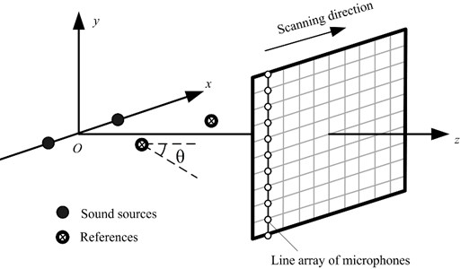
A sound field, generated by two incoherent monopole sources, was investigated to examine the performance of the proposed method using particle velocity references for partial field decomposition. As shown in Fig. 1, two monopole sources were located at the points (–0.25 m, 0, 0) and (0.25 m, 0, 0), respectively. At two points (–0.25 m, 0, 0.05 m) and (0.25 m, 0, 0.05 m) near the sources, the -directional particle velocities were measured as the reference signals, and also the pressures were measured simultaneously to take the role of reference signals for comparison. Here, the pressures and particle velocities are calculated by using Green’s functions of pressure and particle velocity for monopole sources. A line array, composed of 21 microphones, was used to scan the measurement plane, which was 0.1 m away from the source plane. The dimensions of the measurement plane were 1 m×1 m with the sampling interval of 0.05 m in both and directions. To simulate the incoherent relation between the two monopole sources under the scanning situation, a series of random value pairs (respectively indicating the two monopole sources) within , deemed to be the initial phases, were added to the phases of reference and field pressure signals. Note that the initial phase pair added to the field pressures signals and that added to the reference signals were identical per sampling per scan. Here, 50 samples were considered per scan. In addition, white noise with a signal-to-noise ratio of 20 dB was added to the measured signals.
Fig. 1The schematic diagram of numerical simulations
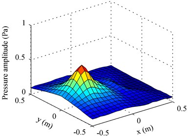
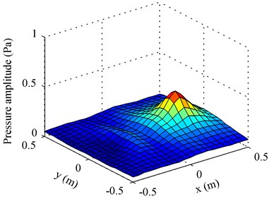
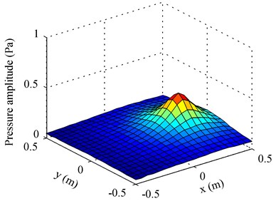
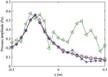
By employing the proposed method using particle velocity references as well as the method using pressure references, the measured sound field at 1000 Hz was decomposed into two partial fields, given in Fig. 2. It can be seen that the decomposed pressures obtained when using particle velocity references are affected less by the other source than those obtained when using pressure references. To show their difference more clearly, the decomposed pressures in the middle line along the -axis on the measurement plane were given in Fig. 3, and the theoretical value was also given in this figure for comparison. Here, the theoretical value of each partial field was obtained by only turning on the corresponding source. From Fig. 3, it can be seen that the decomposed pressures obtained when using particle velocity references agree well with the theoretical values, but the decomposed pressures obtained when using pressure references have a little deviation from the theoretical values near the position where the other source is located. The reason why the particle velocity references outperform the pressure references is that the particle velocity decays more quickly than the pressure when propagating and the particle velocity is a vector. Because of the rapid attenuation of the particle velocity, the particle velocity sensor receives much less information of the source than the pressure sensor when the sensors are placed at the same field point far away from the source. On this basis, the measured particle velocity becomes even smaller because the particle velocity sensor only receives the particle velocity component in the direction under measurement. All in all, the particle velocity reference mainly contains the information of the source close to it and contains little information of the source far away from it. In other words, each particle velocity reference can sense one independent source better than each pressure reference. Thus, the particle velocity references perform better than the pressure references when they are used to realize the partial field decomposition.
Fig. 2Amplitudes of decomposed pressures on the measurement plane at 1000 Hz: a) First partial field when using pressure references; b) second partial field when using pressure references; c) first partial field when using particle velocity references; d) second partial field when using particle velocity references
a)
b)

c)
d)
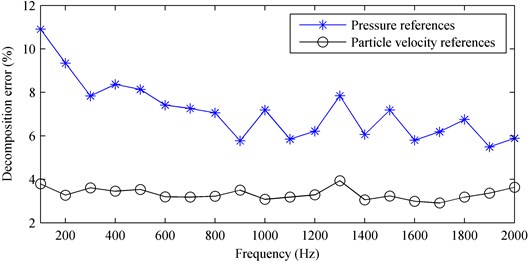
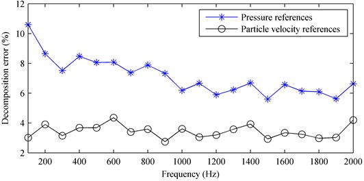
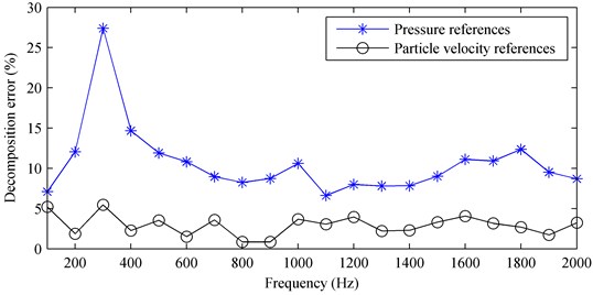
In order to further verify the improvement of the performance of the proposed method using particle velocity references instead of pressure references, Fig. 4 gives the decomposition error at a frequency range from 100 Hz to 2000 Hz. Here, the decomposition error was defined as:
where denotes the decomposed pressures shown in Fig. 2 and denotes the corresponding theoretical ones. From Fig. 4, it can be seen that the decomposition error obtained when using particle velocity references is smaller than that obtained when using pressure references, showing that the particle velocity is more suitable to be used as references than the pressure.
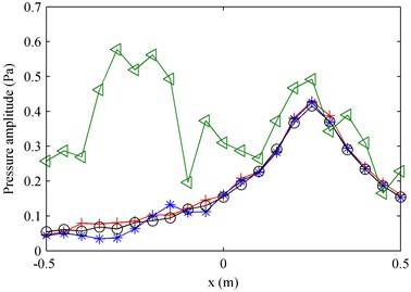
Fig. 3The comparison of amplitudes of pressures in the middle line along the x-axis on the measurement plane at 1000 Hz: a) first partial field; b) second partial field. ◁ – Total pressure; + – theoretical pressure (the two theoretical values presented in the two subfigures respectively represent the pressures radiated by the two sources); * – decomposed pressure when using pressure references; o – decomposed pressure when using particle velocity references
a)
b)
Fig. 4The decomposition error versus the frequency: a) first partial field; b) second partial field
a)
b)
3.2. Influences of reference locations and directions of particle velocity references
The accuracy of partial field decomposition highly depends on the reference locations when pressures are used as references [9-12]. In this section, the influence of the locations of particle velocity references on the decomposition accuracy was investigated. The directions of particle velocity references were also taken into account because the particle velocity is a vector. Here, the direction was represented by the angle deviating from the -axis and the particle velocity sensor is rotating from the -axis to the -axis in the plane with the increase of the angle , as shown in Fig. 1.
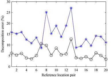
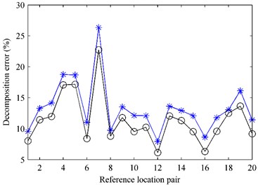
Figs. 5 gives 20 pairs of reference locations which were selected randomly from two areas, (–0.35 m –0.15 m, –0.15 m 0.15 m, 0.05 m) and (0.15 m 0.35 m, –0.15 m 0.15 m, 0.05 m), covering the two sources, respectively. And the reference locations are numbered. However, some references were located at the same positions due to random selection. To avoid the confusion caused by overlapping numbers, some numbers of the reference locations were not shown in Fig. 5 and they are given in Table 1. Meantime the corresponding numbers of reference locations with the same positions shown in Fig. 5 were also given in Table 1. By placing the two references at the reference location pair sequentially, the decomposition error at 1000 Hz when using particle velocity references as well as that when using pressure references were obtained and given in Fig. 6. Note that the angle was set as 0° in Fig. 6, i.e., the directions of particle velocity references were parallel to the -axis and perpendicular to the source plane. From the figure, it can be found that the locations of particle velocity references have more or less influence on the decomposition accuracy but they affect the decomposition accuracy less than those of pressure references, and the decomposition error when using particle velocity references is almost always smaller than that when using pressure references. Observing Fig. 6, it can be found that the decomposition error when using particle velocity references is slightly larger than that when using pressure references on the condition that taking No. 7 reference location to obtain the first partial field and taking No. 1 or No. 8 reference location to obtain the second partial field. From Fig. 5, it is easily to find that No. 7 reference location was just at the corner far away from the first source and No. 1 and No. 8 reference location were just at the corner far away from the second source.
Fig. 520 pairs of reference locations. ⨁ – sources; ○ with number inside: references
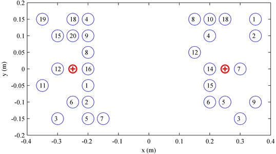
Fig. 6The decomposition error versus the reference location pair at 1000 Hz: a) first partial field; b) second partial field. * – pressure references; o – particle velocity references in the case that the angle was set as θ = 0°
a)
b)
Table 1Numbers of reference locations with the same positions
Area | Not shown in Fig. 5 | Shown in Fig. 5 |
Negative half of -axis | No. 10 | No. 6 |
No. 13 | No. 2 | |
No. 14 | No. 9 | |
No. 17 | No. 6 | |
Positive half of -axis | No. 11 | No. 3 |
No. 13 | No. 8 | |
No. 16 | No. 6 | |
No. 17 | No. 15 | |
No. 19 | No. 18 | |
No. 20 | No. 5 |
Fig. 7 shows the decomposition error versus the angle at 1000 Hz when using particle velocity references whose locations are the same as those in Sec. 3.1. It can be seen that the decomposition error increases with the increase of the angle . When the angle 50°, the partial field decomposition is very successful with the largest error of 6.38 %, but the decomposition fails when the angle is up to 90°. This is because the references mainly contain the information of the source close to them in the case 0°, contain less and less information of the source close to them but more and more information of the source far from them when the angle increases, and finally contain almost only the information of the source far from them in the case 90°. Inspired by this interesting phenomenon, the two decomposed partial fields may be exchanged in the case 90°, then the partial field decomposition could get a good accuracy, 2.47 % for the first partial field and 4.59 % for the second partial field. However, it should be stated that this exchange is invalid if the number of sources is more than two. In summary, the directions of particle velocity references should try to be perpendicular to the source plane, i.e., the angle should be as small as possible, to obtain much better decomposition accuracy.
Fig. 7The decomposition error versus the angle θ at 1000 Hz. □ – First partial field; ☆ – second partial field
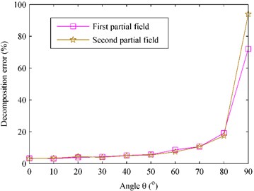
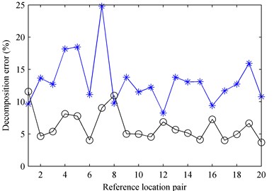
Fig. 8 gives the decomposition error when using particle velocity references as a function of both the reference location pair and the angle at 1000 Hz. It is expectable that the decomposition error varies randomly with the reference location pairs and increases with the increase of the angle . Selecting the case that the angle was set as 50°, the decomposition error versus the reference location pair was shown in Fig. 9. The decomposition error versus the reference location pair when using pressure references, presented in Fig. 6, was also shown in Fig. 10 for comparison. It can be seen that the decomposition error when using particle velocity references is slightly smaller than that when using pressure references no matter where the references are placed, even though the angle is rather large up to 50°. Fig. 10 gives the decomposition error versus the angle in the case that the two references were located at a random reference location pair, e.g., the 10th reference location pair [(–0.25 m, –0.1 m, 0.05 m) and (0.2 m, 0.15 m, 0.05 m)], where the decomposition errors when using pressure references shown in Fig. 6 are 19.44 % for the first partial field and 11.67 % for the second partial field. From Fig. 10, it can be seen that the decomposition errors are all smaller than 19.44 % for the first partial field plotted by the dashed line and 11.67 % for the second partial field plotted by the dotted line, showing the better performance of particle velocity references over the pressure references. Fig. 10 also shows a beneficial conclusion that the particle velocity references can obtain good accuracy even for the case 90° as long as the locations of references have a little offset from the sources along or directions.
Fig. 8The decomposition error versus the reference location pair and the angle θ at 1000 Hz: a) first partial field; b) second partial field
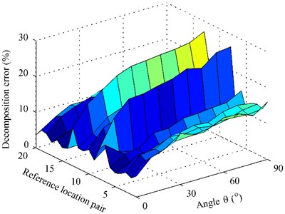
a)
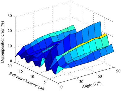
b)
Fig. 9The decomposition error versus the reference location pair at 1000 Hz: a) first partial field; b) second partial field. * – pressure references; ○ – particle velocity references in the case that the angle was set as θ= 50°
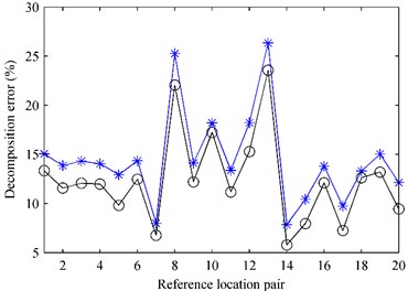
a)
b)
4. Experiment
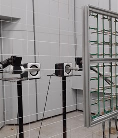
An experiment with two loudspeakers was carried out in a semi-anechoic chamber, as shown in Fig. 11. According to the coordinate system in Fig. 1, two speakers were placed at the points (–0.05 m, 0, 0) and (0.1 m, 0, 0), respectively. To obtain the particle velocity reference signals and pressure reference signals, two - probes produced by Microflown Technologies were placed in the adjacent area of the two speakers with their coordinates of (–0.05 m, 0, 0.05 m) and (0.1 m, 0, 0.05 m), respectively, and particle velocity sensors were placed with their directions parallel to the direction as far as possible. The measurement plane was located at 0.1 m. An array, consisting of 5×7 microphones with the interval of 0.05 m in both and directions, was used to scan the measurement plane. By scanning three times along the direction, 15×7 measurement points were included, and thus an area of 0.7 m×0.3 m was covered.
Fig. 10The decomposition error versus the angle θ at 1000 Hz in the case that the two references were located at the 10th reference location pair [(–0.25 m, –0.1 m) and (0.2 m, 0.15 m)]. The dashed line represents the decomposition error of the first partial field when using pressure references, and the dotted line represents the decomposition error of the second partial field when using pressure references. □ – First partial field; ☆ – second partial field
![The decomposition error versus the angle θ at 1000 Hz in the case that the two references were located at the 10th reference location pair [(–0.25 m, –0.1 m) and (0.2 m, 0.15 m)]. The dashed line represents the decomposition error of the first partial field when using pressure references, and the dotted line represents the decomposition error of the second partial field when using pressure references. □ – First partial field; ☆ – second partial field](https://static-01.extrica.com/articles/21201/21201-img18.jpg)
The sampling frequency was 10240 Hz and the number of measurement repetitions per scan was 30. The signals used to drive the two speakers were synthesized by using a series of sinusoidal signals with the frequency range from 100 to 2000 Hz and the frequency interval of 100 Hz. To simulate two incoherent sound sources, two computers were used to generate two independent signals to drive the two speakers and the two signals were regenerated per sampling per scan.
Fig. 11Photograph of the experimental setup
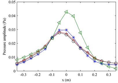
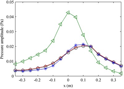
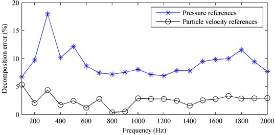
By employing the proposed method using particle velocity references and the method using pressure references, the two partial fields were decomposed from the measured sound field at 1000 Hz. The result shows that both the two methods can realize the partial field decomposition well, but the decomposed pressures they obtained show a small difference. In order to show their difference more clearly, Fig. 12 gives the decomposed pressures and their corresponding theoretical values in the middle line along the -axis on the measurement plane at 1000 Hz. Here, the theoretical values were measured by turning on one speaker and turning off the other as done in numerical simulations. It can be seen that the decomposed result when using particle velocity references agrees better with the theoretical value than that when using pressure references. Figure 13 shows the decomposition error versus the frequency. It further demonstrates that the proposed method using particle velocity references has higher accuracy than the method using pressure references.
Fig. 12The comparison of amplitudes of pressures in the middle line along the x-axis on the measurement plane at 1000 Hz: a) first partial field; b) second partial field. ◁ – Total pressure; + – theoretical pressure (the two theoretical values presented in the two subfigures respectively represent the pressures radiated by the two loudspeakers); * – decomposed pressure when using pressure references; o – decomposed pressure when using particle velocity references.
a)
b)
Fig. 13The decomposition error versus the frequency: a) first partial field; b) second partial field
a)
b)
5. Conclusions
This paper puts forward to use the particle velocity as references instead of pressure in the partial field decomposition method to decompose the sound field radiated by incoherent or partially coherent sources into mutually incoherent partial fields. Because the particle velocity decays more quickly than the pressure when propagating and the particle velocity is a vector, it is expected that each particle velocity reference could sense one independent source close to it better than each pressure reference and the partial field decomposition using particle velocity references could work better than that using pressure references. Both numerical and experimental results confirm the superiority of the proposed method using particle velocity references over the method using pressure references. Moreover, the influences of reference locations and directions of particle velocity references on the decomposition accuracy were also investigated through numerical simulation. It is found that the particle velocity references generally perform better with smaller decomposition error than the pressure references at the same reference locations, but the decomposition accuracy when using particle velocity references is more or less sensitive to their directions because the particle velocity is a vector. According to numerical results, the directions of particle velocity references should try to be perpendicular to the source plane as far as possible to ensure good decomposition accuracy. Fortunately, even though the angle between the -axis and the direction of particle velocity approaches to 50°, the particle velocity references still perform better than the pressure references. When the references are not just placed in front of the sources but in the adjacent area of the sources, the proposed method using particle velocity references can obtain especially good decomposition accuracy, even in the case that 90°. Thus, the particle velocity deserves recommendation as references for partial field decomposition.
References
-
Williams E. G. Fourier Acoustics: Sound Radiation and Nearfield Acoustical Holography. Academic Press, San Diego, 1999.
-
Geng L., Yu L., He C. D., Wang W. G. A multistep acoustic method for suppressing the reconstruction instability of instantaneous vibration of an exciting planar structure. Mechanical Systems and Signal Processing, Vol. 135, 2020, p. 106402.
-
Tan D. Y., Chu Z. G., Wu G. J. Robust reconstruction of equivalent source method based near-field acoustic holography using an alternative regularization parameter determination approach. Journal of the Acoustical Society of America, Vol. 146, Issue 1, 2019, p. 34-38.
-
Hald J. STSF – A Unique Technique for Scan-Based Near-Field Acoustic Holography Without Restrictions on Coherence. B&K Technique Review, 1989.
-
Bendat J. S., Piersol A. G. Random data: Analysis and Measurement Procedures. 4th Edition, Wiley and Sons, Hoboken, 2010.
-
Hallman D., Bolton J. S. Multi-reference nearfield acoustical holography. Proceedings of Inter-Noise, Toronto, Canada, 1992, p. 1165-1170.
-
Tomlinson M. A. Partial source discrimination in near field acoustic holography. Applied Acoustics, Vol. 57, Issue 3, 1999, p. 243-261.
-
Nam K. U., Kim Y. H. A partial field decomposition algorithm and its examples for near-field acoustic holography. Journal of the Acoustical Society of America, Vol. 116, Issue 1, 2004, p. 172-185.
-
Kim Y. J., Bolton J. S., Kwon H. S. Partial sound field decomposition in multireference near-field acoustical holography by using optimally located virtual references. Journal of the Acoustical Society of America, Vol. 115, Issue 4, 2004, p. 1641-1652.
-
Wall A. T., Gardner M. D., Gee K. L. Coherence length as a figure of merit in multireference near-field acoustical holography. Journal of the Acoustical Society of America, Vol. 132, Issue 3, 2012, p. 215-221.
-
Kwon H. S., Kim Y. J., Bolton J. S. Compensation for source nonstationarity in multireference scan-based near-field acoustical holography. Journal of the Acoustical Society of America, Vol. 113, Issue 1, 2003, p. 360-368.
-
Chen Z. M., Zhu H. C., Mao R. F. Partial field decomposition of multi-source cyclostationary sound field. Applied Acoustics, Vol. 73, Issue 5, 2012, p. 524-528.
-
Lee M., Bolton J. S., Mongeau L. Application of cylindrical near-field acoustical holography to the visualization of aeroacoustic sources. Journal of the Acoustical Society of America, Vol. 114, Issue 2, 2003, p. 842-858.
-
Lee M., Bolton J. S. Scan-based near-field acoustical holography and partial field decomposition in the presence of noise and source level variation. Journal of the Acoustical Society of America, Vol. 119, Issue 1, 2006, p. 382-393.
-
Kang Y. J., Hwang E. S. Beamforming-based partial field decomposition in NAH. Journal of Sound and Vibration, Vol. 314, Issues 3-5, 2008, p. 867-884.
-
Takata H., Nishi T., Jiang W., J Bolton. S. The use of nearfield acoustical holography (NAH) and partial-field decomposition to identify and quantify the sources of exterior noise radiated from a vehicle. Journal of the Acoustical Society of America, Vol. 100, 1996, p. 2654-2655.
-
Wall A. T., Gee K. L., Neilsen T. B., McKinley R. L., James M. M. Military jet noise source imaging using multisource statistically optimized near-field acoustical holography. Journal of the Acoustical Society of America, Vol. 139, Issue 4, 2016, p. 1938-1950.
-
Wall A. T, Gee K. L., Leete K. M. Partial-field decomposition analysis of full-scale supersonic jet noise using optimized-location virtual references. Journal of the Acoustical Society of America, Vol. 144, Issue 3, 2018, p. 1356-1367.
-
Leete K. M., Gee K. L., Liu J. H., Wall A. T. Partial field decomposition of the simulated noise from a highly heated laboratory-scale jet. Journal of the Acoustical Society of America, Vol. 146, Issue 4, 2019, p. 3042.
-
Bi C. X., Guo M. J., Zhang Y. B., Xu L. Partial field decomposition using pressure gradient references. Proceedings of Inter-Noise 2012, New York, America, 2012, p. 2214-2225.
-
Bi C. X., Guo M. J., Zhang Y. B., Xu L. An investigation of partial field decomposition using pressure gradient reference. Acta Physica Sinica-Chinese Edition, Vol. 61, Issue 15, 2012, p. 415-418.
About this article

This work was supported by the National Natural Science Foundation of China (Grant No. 11704110), Major Fund Project of Technical Innovation in Hubei (2017AAA133); Hubei Superior and Distinctive Discipline Group of “Mechatronics and Automobiles” (XKQ2020010). The authors would like to thank Microflown Technologies for lending us a sound intensity probe.
