Fault detection method based on an automated operating envelope during transient states for the large turbomachinery

1. Introduction

In the energy generation business steam powered turbo-generators still play an important role in electrical power generation all over the world. The survey by Xiao et al. [1] presents the main components of a fossil-fuel power plant (FFPP) and its importance as well as its share in the world power generation industry.

The renewable power generation grows significantly, especially in recent years [2], but it is still not sufficient as a sole energy source suitable for a heavy industry and must be supported by other sources [3]. All large facilities and factories require electric power to be generated in the most reliable way. Up to now, large turbo-sets play such a role. A particular example of such arrangement is a steam turbine coupled with a generator. The 200 MW type steam turbine unit is the most popular one in Poland power generation industry [2]. Such a unit must be operated continuously for a long time. Extensive research carried out by the German insurance company Allianz and gathered in [4] revealed a number of examples of lack of proper diagnostics and its consequences, leading in extreme cases to total machine destruction. As new diagnostic technologies are being developed, e.g. state-of-the-art thermal and flow diagnostic of steam turbines (described by Głuch in chapter 3 of [5]) and introduced to power plants, still vibration response of the unit remains the fundamental method to assess the technical state of turbo-sets. In [6] authors perform analysis of a complex case of Gas Turbine vibrations. They confirm the fact that tedious analysis work and availability of experts is required for proper detection and identification of a large turbomachinery fault.

Together with the industry 4.0 concept new challenges arise both for the machines which are expected to be more reliable and for monitored data to properly diagnose malfunction without the need of expert knowledge. Lis in [7] proposed a concept of novelty detection method in time domain for an over-hung centrifugal pumps to meet such a demand.

Sometimes the interval between shutdowns can be several months, or even longer. During this period the turbo-set is operated in varying conditions such as load change from 40 % up to nominal load, different steam temperatures and pressures. This type of operation can introduce large amount of stress, which eventually can lead to fatigue and, in an extreme cases, to a failure. Zagorowska et al. [8] presented interesting approach and new insights to track an evolution of malfunction during steady-state operation with novel approach to trend tracking technic. There are a lot of works dedicated to fault diagnosis of bearings. Wei et al. [9] used adaptive approach to extract features from faulty bearings with success. Kun et al. [10] has proposed also interesting approach to bearing faults classification. Authors used Ensemble Empirical Mode Decomposition (EEMD) and Singular Value Decomposition (SVD) to extract fault features and then used advanced clustering method for fault pattern recognition. Wang et al. [11] used also ML technics and incorporated them to planetary gearbox malfunctions detection. The papers mentioned above studied only machines with rolling element bearings or planetary gears during their steady state operation. Duan et. al in [12] presented several attempts of tracking turbogenerator degradation with Deep Neural Networks. The features however were calculated from turbo-set operation data not during transient states. An interesting approach to bearing diagnosis was introduced by Sachin et al. [13]. It proposes reducing the number of feature. Authors showed that proper feature ordering and selection can significantly improve the classification accuracy especially for machines which are equipped in modern CMS which acquire and calculate huge amount of features

The best industrial practice is to assess machine dynamic state during each and every transient state operation, i.e. a shutdown and a start-up. Data from these states carry much more information than from operation at a constant rotational speed but they can also suffer from higher distortion.

Assessment and comparison of data from different transient states is not an easy and straightforward task as shown in [14]. During transient a machine can be susceptible to a number of potentially harmful events. Main malfunctions which can be much easier diagnosed during transients are (according to [15], [14], [16] and [17]):

– Excessive unbalance.

– Misalignment.

– Resonances.

– Rubs (which can occur both during steady state operation, or can develop during shut-downs/start-ups).

The automated assessment of complex technical systems was subject of numerous research. Demetul et al. in [18], highlight the fact that most industrial systems are non-linear and require appropriate analysis methods. Each such an attempt must include feature extractor and classifier. The authors have analyzed multiple generic methods for the diagnostic of the pneumatic systems of the material handling systems, starting from dimension reduction to clustering for classification.

Proper diagnostics of turbomachinery requires a skilled expert and a large amount of knowledge. For instance, the mathematical background and dynamics of listed malfunctions is well described by Muszyńska in [16] and by Ehrich in [19]. Practical procedures and techniques are presented e.g. in [14], [20] and [21]. Those combined with mathematical and mechanical background presented in [16]-[21] is the way to fully assess machine’s dynamic state and try to troubleshoot problems which these machines can suffer from. Models for analyzing large turbogenerator behavior can be extremely complex. FEM model was used by Kiciński in [22] to replicate the behavior of the +200 MW turbo-set. However, there is often no such personnel at hand and a lot of information of machine’s technical state goes without analysis. Maintenance and operation personnel have not enough qualifications, skills and knowledge to carry out such a complex task. To properly assess various parameters during those events professional knowledge and experience are needed.

There is a lack of the method to help the maintenance personnel to quickly assess the state of machinery during turbine cast-downs and start-ups, ideally in an automated way. The authors in [4] showed that such a method will be very helpful and can be beneficial in two ways: as a “health monitoring” parameter for the maintenance personnel and for the planner and management personnel – to properly plan and execute machine’s inspections and overhauls. In [23] Bornassi et al. highlighted the importance of analysis of transients states in case of large turbomachinery blades. Authors in the paper presented combination of 1DOF model with real blade vibration measurement data to identify the vibration parameters of blades during transient state. Therefore, creation of a method to define a healthy pattern (i.e. baseline or reference) is of a great value. Having such a pattern, together with some acceptance boundaries, they can compare each transient whether it represents a healthy condition. Due to lack of skilled personnel, it should be reiterated that the method should be automated. The authors proposed such a method and coined a name Operational Envelope (OpEn). This idea is based on an envelope wrapped around 1st harmonic amplitude during the transient state of the machine.

The paper is organized as follows. Section 1 presents introduction to the paper. Section 2 depicts a brief description of the method used to achieve the center of the Operating Envelope. We present a flow chart of the whole process beginning with data acquisition to the final presentation. Additionally, criteria for quantitative assessment of deviation from the healthy state – called malfunction severity parameters – were proposed. In Section 3 we present a case study, based on a 200 MW type unit in one of Polish power plants. In Section 4 we present and discuss our findings based on the case study. As a conclusion of this paper we point out further steps we plan to undertake in order to extend our method across the entire shaft line.

Main novelty of the paper is the automated method for novelty detection of machine’s vibration. Vast majority of previously proposed methods apply to smaller machines with rolling bearings. The method we propose can be applied to large power generation machines, which have very different dynamic behavior. First, they are equipped with sliding bearings, which have highly non-linear characteristics and may exhibit unique malfunctions, e.g. oil film instabilities. Second, large machines operate over the first (sometimes even second) critical speeds and novelty detection method must be able to tackle the resonance data.

2. Description of the method

This section describes the Operational Envelope (OpEn) method in detail. The method consists of several steps. First, we collected real data from the transient state of the tubine-generator set. Then we used the acquired data and data from the turbine’s design (from GE engineering department) to determine the baseline transient which suit the best to the design one. Next we processed this baseline transient with the Cubic Spline interpolation to have equally distributed data points across whole rotational speed range and to establish the center of OpEn, and then its upper and lower values. The OpEn together with upper and lower bonds create the acceptance region and from now on, new data can be quickly verified if it is inside this region. If the all the data from a new transient state, are contained within the OpEn – no further improvement actions are required. However, if the data (or a few points from the transient) are outside the OpEn, then further actions should be suggested to assess severity of the malfunction.

In our paper we have coined the name of the “operational envelope” which describes the meaning of the actions involved, but the reader should not mistakenly mixed it with the concept of the “signal envelope” and its spectrum, called “Envelope Spectrum”. These are two different methods and there are several significant differences between the spectrum envelope and the Operational Envelope proposed in this paper. Table 1 summarizes main differences between these two concepts.

We consider each sampled datapoint gathered during coast down or start-up as an amplitude of a single line from the spectrum, then accompanied by an acceptance region, i.e. upper and lower bounds – in other words – enveloped. The method is implemented only for transient states which require change of the rotational speed. That is why the domain of OpEn is rpm/cpm (revolutions/cycles per minute) and not Hz with a constant rotational speed. The Envelope Spectrum is calculated from the signal envelope and is the established technique for detection e.g. of Rolling Element Bearing faults.

Fig. 1Flow chart of OpEn method

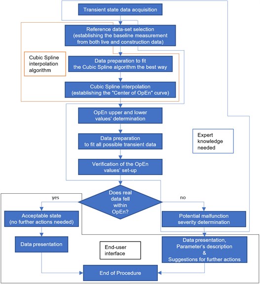
Fig. 1 depicts the OpEn method, together with division of the most important parts of program. In following sections we will describe the key steps of our method.

2.1. Cubic spline preprocessing

In order to properly assess the data gathered during transients states, the measurement data should be properly acquired and preprocessed before they can be useful. Data are measured and collected/acquired by different systems, having different resolutions (it especially applies to the rotational speed). Collected data cannot be directly compared and needs pre-processing. It can be compared amplitude-wise (comparing amplitudes from one transient with another). This method is not practical to be implemented in our case. Depending on triggers setting, the data will be recorded for very different rpms. If one compares the amplitudes from different rpms, such an analysis will be misleading. More advanced (and useful) type of analysis is to assess transient data signals, but with respect to a reference mark which is the same for all analyzed transient states. We assume that such a mark is the rotational speed. Choosing rotational speed mark as the reference signal enables to compare data in repetitive and reliable way. Data prior, during and past critical speed can be unequivocally identified and compared. Resonance peaks and unbalance response are only a few out of many, which highly depends on rotational speed which should be appropriately compared, independently on a trigger setting.

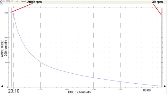
Gathering sufficient amount of data during transient states requires using two kinds of triggers: one is rotational speed-depended, and the other one is time-depended. Fig. 2 presents inertia of the system during a typical cast down. It is visible that starting from the trip point (at the full rotational speed of the machine) goes down to approx. 1/6 of nominal speed (500 revolutions per minute) rotational speed changes quickly in comparison to time. That is why during the “first stage” of a coast-down a rpm-dependent trigger plays greater role. During the “second stage” rotational speed changes are not so significant comparing to the time. On that stage more samples (i.e. information) will be provided by the time-dependent trigger. Such complicated trigger procedure generates a different set of samples every time a transient is recorded. Data points are placed close to each other (comparing transient-to-transient), but not identically with respect to rotational speed mark.

Due to the fact that acquired data are field measurements and also that we measured many machines (of the same type, but still different units), the noise reduction was also an important matter. We used the Cubic Spline method for both tasks.

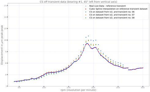
Sampling data unequally spaced along the rotational speed axis can introduce a lot of difficulties in implementation of processing algorithms. In order to tackle this issue we support the idea that it is necessary to convert the data to the rpm-equidistant model. We have to start from a function which creates an equally spaced vector of rotational speeds along each particular transient. In other words, the first step is resampling of the speed vector to generate a data vector having the same rpm values for all the transients. Thus, CS function helps to generate data points for the same rotational speed points. It must also handle “cropped” transients, i.e. transients which do not start at 0 rpm and finishes at the FSNL (Full Speed No Load) point. The Fig. 2 presents “reference transient” with all the actual data (blue line), and its CS interpolation – blue dots at every 50 rpm interval. It is apparent that CS results from other two example transients (no. 6 and no. 7) are located in the same places on rotational axis as our CS from the reference transient. Advantages of equally spaced points/knots in polynomial spline functions are presented in [24] and in [25].

The Cubic Spline interpolation is a type of interpolation which well handles the problem of oscillating edges of intervals with equally spaced interpolation points when using higher order polynomial interpolation. Theoretical considerations and applications were described by Gerald and Wheatley in [26].

Fig. 2Revolutions per minute in respect to time during typical transient state (cast down example)

Schumaker in [25] formulated a set of four general properties for a centerline of the cubic spline function $s$ in the Carteisan plane for a set of points $\left(x_i,y_i\right)$, $i=\mathrm{1,2},\dots ,k$:

1) $s$ is a piecewise cubic polynominal with knots at $x_1,\dots ,x_k$.

2) $s$ is a linear polynomial for $x\le x_1$ and $x\ge x_k$.

3) $s$ has two continuous derivatives everywhere.

4) $s\left(x_i\right)=y_i$, $i=\mathrm{1,2},\dots ,k$.

Such function produces less error and improves accuracy. The theory together with a process of creating and using of spline is shown in [24] and [26]. A few examples with using a spline interpolation as a curve fitting aid are shown in [25].

Fig. 3Equally spaced CS interpolation for reference and regular transiens datasets.

The main idea of cubic spline is presented by Schumaker in [24]. The goal is to produce a set of the third degree polynomial functions $s_i\left(x\right)$ that satisfy:

1

$S\left(x\right)=\left\{\begin{array}{ll}{s}_1\left(x\right),& x_1\le x<x_2,\\ s_2\left(x\right),& x_2\le x<x_3,\\ ⋮& \\ s_{n-1}\left(x\right),& x_{n-1}\le x<x_n.\end{array}\right.$

Where polynomial to be fitted across each interval $x_i\le x<x_{i+1}$, is given by equation:

2

$s_i\left(x\right)=a_i{(x-x_i)}^3+b_i{(x-x_i)}^2+c_i\left(x-x_i\right)+d_i,$

where $i=1,2,\dots ,n-1$, and respectively, the first and the second derivative is given by:

3

$s_i^{\text{'}}\left(x\right)=3a_i{\left(x-x_i\right)}^2+{2b}_i\left(x-x_i\right)+c_i,$

4

$s_i^{\text{'}\text{'}}\left(x\right)=6a_i\left(x-x_i\right)+{2b}_i,$

for the same $i=1,2,\dots ,n-1$.

The matrix equation for the cubic spline interpolation is given by:

5

$\left[\begin{array}{ccc}\begin{array}{cc}1& 4\\ 0& 1\\ 0& 0\end{array}\begin{array}{cc}1& 0\\ 4& 1\\ 1& 4\end{array}& \cdots & \begin{array}{cc}0& 0\\ 0& 0\\ 0& 0\end{array}\begin{array}{cc}0& 0\\ 0& 0\\ 0& 0\end{array}\\ ⋮& \ddots & ⋮\\ \begin{array}{cc}0& 0\\ 0& 0\\ 0& 0\end{array}\begin{array}{cc}0& 0\\ 0& 0\\ 0& 0\end{array}& \cdots & \begin{array}{cc}4& 1\\ 1& 4\\ 0& 1\end{array}\begin{array}{cc}0& 0\\ 1& 0\\ 4& 1\end{array}\end{array}\right]\left[\begin{array}{c}\begin{array}{c}{M}_1\\ M_2\end{array}\\ M_3\\ M_4\\ ⋮\\ M_{n-3}\\ M_{n-2}\\ M_{n-1}\\ M_n\end{array}\right]=\frac{6}{h^2}\left[\begin{array}{c}{y}_1-2y_2+y_3\\ y_2-2y_3+y_4\\ y_3-2y_4+y_5\\ ⋮\\ y_{n-4}-2y_{n-3}+y_{n-2}\\ y_{n-3}-2y_{n-2}+y_{n-1}\\ y_{n-2}-2y_{n-1}+y_n\end{array}\right],$

where: $M_i=s\mathrm{\text{'}}\mathrm{\text{'}}\left(x_i\right)$, and $h={x_i-\mathrm{}x}_{i-1}$.

This is an under-determined system ($n-2$ rows by $n$ columns). To find unique solutions for the matrix Eq. (5) the following assumptions has to be made:

1) $M_1=2{M_2-M}_3$.

2) $M_N=2{M_{N-1}-M}_{N-2}$.

This boundary conditions let us reduce the system matrix to a $n-2$ by $n-2$ dimensions:

6

$\left[\begin{array}{ccc}\begin{array}{ccc}6& 0& 0\\ 1& 4& 1\\ 0& 1& 4\end{array}& \cdots & \begin{array}{ccc}0& 0& 0\\ 0& 0& 0\\ 0& 0& 0\end{array}\\ ⋮& \ddots & ⋮\\ \begin{array}{ccc}0& 0& 0\\ 0& 0& 0\\ 0& 0& 0\end{array}& \cdots & \begin{array}{ccc}4& 1& 0\\ 1& 4& 1\\ 0& 0& 6\end{array}\end{array}\right]\left[\begin{array}{c}{M}_2\\ M_3\\ M_4\\ ⋮\\ M_{n-3}\\ M_{n-2}\\ M_{n-1}\end{array}\right]=\frac{6}{h^2}\left[\begin{array}{c}{y}_1-2y_2+y_3\\ y_2-2y_3+y_4\\ y_3-2y_4+y_5\\ ⋮\\ y_{n-4}-2y_{n-3}+y_{n-2}\\ y_{n-3}-2y_{n-2}+y_{n-1}\\ y_{n-2}-2y_{n-1}+y_n\end{array}\right].$

Solving Eq. (6) yields the sought equally distanced interpolated data points.

2.2. Upper and lower values for OpEn definition

Setting up an upper and lower bounds for the OpEn is not a trivial task. The bounds mean the actual Operational Envelope above and below the centerline calculated as described in the previous section. We expect transients measured on healthy machines to stay within the area between lower and upper bounds.

Vance throughout its book [20] studied how different setups of the bearing applied to the same machine can produce dramatically different results. Eisenmann in [21] well described and explained how damping and stiffness affect response of the system during transient states. Thus, one needs to be aware of large effects caused by small changes.

The upper value should be set up higher, because of the non-linear nature of damping in bearing-rotor system as explained in [14]-[21] and [11]. For instance, having properly aligned and balanced rotors on the same machine, different state of initial conditions (such as rotor and/or steam temperature, time of stand-still, etc.) can cause higher amplitudes, especially when whirling speed approaches to the resonant speed. Similarly, differences in inlet oil temperatures can produce differences in resonant peak amplitudes, and this is directly related to the oil damping properties.

The lower values are also important to analyze. The behavior of both static and dynamic response of rotor system changes together with crack propagation. Bachachmid described these phenomena in detail in [27]. Setting up lower value of OpEn can be a great help with shaft crack detection. As was presented in [4], [14], [21] during evolution of a crack in the shaft its stiffness deteriorates. Such a phenomenon causes resonance frequency move to the direction of lower frequencies.

Based on the authors’ experience, reinforced with suggestions from GE’s engineering department we assumed to set up values as follows:

– Upper value of “the Center of OpEn” will be 24 µm_pp.

– Lower value of “the Center of OpEn” will be 13 µm_pp.

Fig. 4OpEn and its upper and lower values.

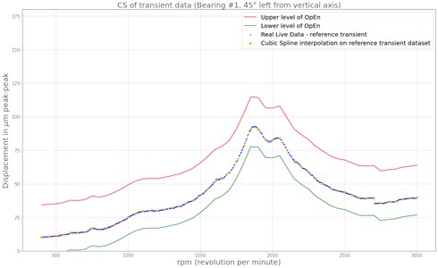
These values create an interval of acceptable amplitudes for each rotational speed throughout whole speed range as it is presented in Fig. 4. They are valid for this particular sensor in this particular unit. As it is initial stage of research, we accept such a “trial-and-error” approach. During further research we will try to develop a general rule for setting these bounds for other sensors and units.

The method should analyze vibrations across large span of rotating speeds. The span depends on the basic characteristics of the machine. For the majority of gas and steam power generation units based in Poland (and most other countries) the span is between 500 and 3000 rpm. It is an obvious consequence of the fact that these units operate at the rotating speed of 3000 rpm (i.e. 50$$Hz). For machines in North and Latin America, it is 500…3600 rpm. Similarly, for hydro power plants, which have multiple pole pairs and thus, lower rotational speeds or high speed turbo-generators, equipped with gears, the range of rotational speeds must match typical operation. The other consideration is the set of available data, as not always the measured transients will have all the rotational speeds in range. It is not unusual that the run-up will not reach the nominal rotational speed, typically due to problems with the dynamic state. The proposed method must be able to accommodate subsets of the rpm range. The only requirement is that the data should cover all the important ranges, for instance resonant speeds.

2.3. Malfunction severity parameters description

The core of the method is detection of anomalies during transient states. The method, which was presented so far, is able to create two vectors having the same rotational speed values and different amplitudes of 1X feature. These vectors define upper and lower bounds of the OpEn. To automate the detection of anomalies it is necessary to define a measure of distance of a new vector from a new transient from the defined OpEn and to propose a threshold. The threshold will classify new vectors as they are measured. Only then the method can be proposed to machinery operators, and they will be able to use it without specialist knowledge and experience.

There is no single “silver bullet” method in order to appropriately assess if a particular vector coming from a transient state is considered to be “good” or “bad”. We proposed a few metrics and compared their performance. It shall be discussed theoretically and then presented in a case study. We have considered following metrics:

– RMSE – Root Mean Square Error from the whole transient.

– KURT – Kurtosis from the whole transient.

– MAX_Oo_OpEn – maximum distance above the OpEn upper value.

– MIN_Oo_OpEn – maximum distance below the OpEn lower value.

RMSE is defined as a root mean square between the CS interpolation of the reference transient (the OpEn centerline) and the real data measured by portable data acquisition system in the field on the same rotational velocity points:

7

${RMSE}_{OpEn}=\sqrt{\left[\sum _{i=l}^u\frac{{\left(y_{{ref\_t}_i}-y_{{live\_t}_i}\right)}^2}{T}\right]},$

where: ${RMSE}_{OpEn}$ – root mean square error of given transient, $y_{ref\_t}$ – “healthy” value (reference transient data – center of OpEn), $y_{live\_t}$ – observed value (newly acquired, real transient data), $\left[l,u\right]$ –rotational speed interval, common for $y_{ref\_t}$ and $y_{live\_t}$, $T$ – number of common samples (samples at the same rotational speed points).

Fig. 5 helps visualizing this norm.

Fig. 5RMSE norm visualization

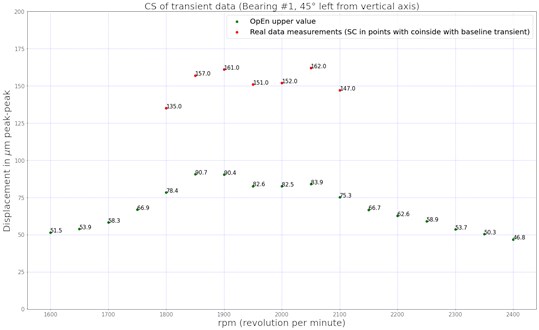
In the example on Fig. 5 above RMSE_OpEn would be:

8

${RMSE}_{OpEn}=\sqrt{\left[\sum _{i=1800}^{2100}\frac{{\left(y_{{ref\_t}_i}-y_{{live\_t}_i}\right)}^2}{7}\right]}.$

RMSE tells us how far on average the newly acquired transient is from the OpEn, where only the centerline is considered. Thus, it a measure of general, average distance between these vectors.

KURT parameter is the fourth standardized moment, and defined as:

9

${KURT}_{OpEn}\left[X\right]=E\left[{\left(\frac{X-\mu }{\sigma }\right)}^4\right]=\frac{E\left[{\left(X-\mu \right)}^4\right]}{{\left(E\right[{(X-\mu )}^2\left]\right)}^2},$

where: $X$ is a vector of real data, $\mu$ is the mean of $X$, $\sigma$ is the standard deviation of $X$.

The KURT parameter represents distance between the two vectors with higher weight of peaks, which should be detected automatically. If a transient differs by a high value at only a few frequencies, it cannot bring sufficient weight to RMSE factor, but will be detected by KURT.

MAX_Oo_OpEn (abbreviation from Maximum Out of Op En) is a measure of the highest distance above the OpEn upper value. As the previous ones, this parameter is measured at common rotational speed values:

10

${\mathrm{M}\mathrm{A}\mathrm{X}}_{Oo\_OpEn}=\mathrm{m}\mathrm{a}\mathrm{x}\left\{abs\left(y_{{OpE{n}_{uv}}_i}-y_{{liv{e}_t}_i}\right)|i\in \left[l,u\right]\right\},$

where: $y_{{OpEn\_uv}_i}$ – OpEn upper bound, ${y_{live\_t}}_i$ – observed value (real transient data acquired during transient), $i\in \left[l,u\right]$ – common rotational speed interval.

As shown in Fig. 6, the maximum value for this transient is 162 µm_pp, and upper value of the OpEn in this rotational speed instance is given as 107.9 µm_pp. So, ${\mathrm{M}\mathrm{A}\mathrm{X}}_{Oo\_OpEn}$ equals 51.1 µm_pp. MAX_Oo_OpEn stays at zero as long as no point from the observed vector protrudes above the upper bound of the OpEn. Thus, it is a quick detection tool, it reacts to any violation of the upper bound.

MIN_Oo_OpEn (abbreviation from Minimum Out of Op En), is symmetrical to the previous measure and it is a measure of the highest distance below the OpEn upper value. Parameter is measured at common rotational speed interval.

11

${MIN}_{Oo\_OpEn}=\mathrm{m}\mathrm{a}\mathrm{x}\left\{abs(y_{{OpEn\_lv}_i}-y_{{liv{e}_t}_i})|i\in \left[l,u\right]\right\}$

where: $y_{{OpEn\_lv}_i}$ – OpEn lower value, ${y_{live\_t}}_i$ – observed value (real transient data acquired during transient), $i\in \left[l,u\right]$ – mutual speed rotation interval.

Fig. 6Plot of “Min Out of OpEn” and “Max Out of OpEn”

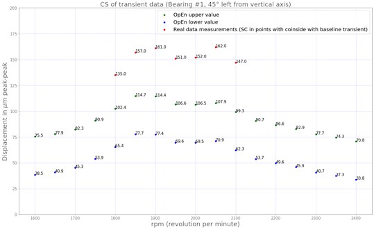
Both MAX_Oo_OpEn and MIN_Oo_OpEn also present the rotational speed value for which the maximum distance was measured. For both methods the result is the maximum distance and the relevant rotational speed.

The list of metrics is not complete and is rather a first set of proposals based on the authors’ experience and engineering practice. To compare its performance a case study will be presented in the next section.

3. Case study

This section will present the example where the transient data signal was acquired from a 13K230 unit in one of the Polish power plants. This type of units have 7 journal bearings and 1 thrust bearing (which is a combi journal-thrust bearing) placed in bearing pedestal no. 2. Schematic picture of this turbo-set in presented in Fig. 7. Normally, these types of machines are equipped in eddy current relative shaft-to-rotor vibration sensors. Typically, all journal bearings in this type of turbines are equipped in such sensors. Every bearing has 2 sensors, oriented perpendicularly to each other. The most common set-up of eddy-current sensors is presented in Fig. 8. Signal from these sensors is proportional to the displacement of the shaft in respect to the bearing housing.

Fig. 713K230 type turbo-generator mechanical component setup

The case study presents the data measured at the bearing no. 1. Measurements were carried out during incremental improvement of the HP-IP part alignment. Data were collected during 10 transient states, both start-ups and cast-downs. Fig. 9 presents all the transients on a single plot. It is worth mentioning that in most cases the coast down transient is better suited for analysis than the run-up, because during this process turbo-set does not experience additional excitation forces. In such a case, machine coast down is driven only by the inertia of the shaft. During the analyzed measurements we did not experience noticeable deviations between start-ups and coast downs. That was a prerequisite for inclusion of start-up into our analysis as well.

Fig. 8Sensor arrangement in bearing

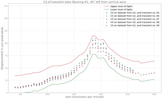
Fig. 9Transient data during measurements course as the machine was incrementally aligned. Transients 01-04 were non-satisfactory. Transients 05-10 were satisfactory. Transient 09 was selected as the reference

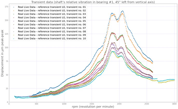
There were no signs of any other malfunction apart from misalignment, as for example rubs which can produce different response of a rotor system during startups and coast-down, as described in various examples, e.g. [14], [16], [21]. We classify the transients in a following way:

– first 2 pairs (transient no. 01-04 in the Fig. 9) of transients are “non-satisfactory” in terms of vibration response,

– next 3 sets of pairs (transients no. 05-10 in the Fig. 9) are “satisfactory” in terms of proper alignment of the HP-IP coupling.

The OpEn centerline was calculated as presented in the Section 2. Upper and lower bounds were set at 24 µm_pp and 13 µm_pp, respectively as explained in Section 2.2. During the first set of transients, the synchronous response exceeded the upper value of OpEn in the [1500, 2600] rotational speed interval. Transient no. 1 and 2 on Fig. 10 depicts this scenario.

Fig. 10Example of a transients with misalignment (the initial state – transient no. 1 and no. 2 and after first improvement – transient no. 3 and no. 4)

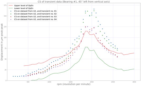
After the first alignment improvement the majority response of rotor system fell into the OpEn. Since start up to approx. 1750 rpm and above 2450 rpm all amplitudes were inside OpEn. Still, the system response values between approx. 1700-2450 rpm had higher values than the OpEn upper bound which can be seen in Fig. 10, transient no. 3 and 4.

Second improvement of the HP-IP cylinder alignment resulted in proper response of the system. This can be seen in Fig. 11.

Fig. 11Example of healthy transients

The figures presented only the qualitative results. To be able to automate the assessment process the parameters proposed in the Section 2.3 were applied and presented in Table 2. The transient no. 09 named “U2_09” was assumed to be the reference one, hence its both RMSE and Kurtosis value in the before last column in Table 2 also named “U2_09” is 0. It is worth underlying that RMSE and Kurtosis values for the last measured transient state named “U2_10” were the lowest ones even though it contained samples from whole rotational speed span (which was > 100 rpm up to 3000 rpm).

Table 2 summarizes performance of the proposed distance criteria. After the second alignment improvement RMSE of further transient in studied case does not exceed value of 10, as shown in Table 2 and since then all amplitudes of synchronous response fell between OpEn upper and lower values.

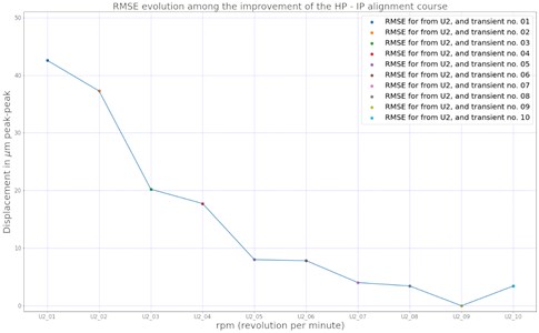
To visualize evolution of RMSE, Fig. 12 represents RMSE error at each transient during measurement course. It is apparent after the forth transient (second HP-IP coupling improvement) dynamic response of the machine is much closer to the reference transient than before.

RMSE is a good parameter as it is sensitive to the distance from the healthy state. As we show in the case study above, it is sensitive to the misalignment level. There is a value above which misalignment is beyond an acceptable level. In the studied example this value should be set at 10 and then it is a good condition indicator (still, for this particular sensor and for this type of malfunction).

Fig. 12Root mean square error (RMSE) evolution vs incremental alignment improvement

Kurtosis parameter is between 2.90 and 1.77. The values do not show the relationship to the level of misalignment. Thus, the Kurtosis parameter is not useful in this case study. In our investigation Kurtosis is the measure how the new transient is similar to its reference one as a shape. It can signal if during particular transient some samples were far off the reference transient. This parameter may play a great role in finding anomalies such as oil whirl or whip. Transient of a machine which experiences such phenomena, can be extremely different form the reference one. Amplitudes generated during instabilities are often close to bearing clearances which can be harmful to turbo-set equipment such as bearing itself, its oil seals, steam seals on the rotor and inside of a turbine casing, hydrogen oil seals (on the generator) and others. The rotational speed intervals in which hydrodynamic instabilities can appear might be narrow comparing to the whole rotational speed range and thus in such cases RMSE as a single assessment parameter of transient cannot suffice, because even if the amplitude of signal is much greater in short interval, the amount of samples in transient as a whole will diminish it.

Setting up the Kurtosis parameter will be a subject of further studies. We will be studying the effect of setting up RMSE and Kurtosis parameters on different signal components in different arrangements, for example RMSE on synchronous response and phase angle and Kurtosis on direct (or sub-synchronous) response.

Max Out of OE well describes misalignment in the studied example. This indicator though, detects if at any given moment during transient state the vibration exceeds the upper OpEn value. This parameter detects if there are any samples which exceed the upper bound and in such a case it returns the distance value and the relevant rotational speed. This parameter presents information about one, „the worst” sample. This parameter can be used to signal abnormal machine behavior during transient, for instance hydrodynamic instability. Thus, the Max Oo OpEn is well suited for novelty detection purposes.

During the presented case study, as shown in Table 2, no transient exceeded the OpEn lower value, so the Min Out of OpEn parameter cannot be evaluated. This can imply two things: one OpEn lover value can be set to too a low value which can cause false positive error (lack of detection in early stage of malfunction evolution), or if misalignment is present in a shaft train there will be no samples with amplitudes lower than expected. This will be the subject of our further studies.

4. Conclusions

Turbo-sets used for power generation are built to long-term operation with as little shut down processes as possible. Sometimes, turbo-set can be operated many months or even a year without a coast down. On the other hand, such a transient situation carries important diagnostic information of a machine condition. Sometimes machine has to be shut down because of some process dependent variables (such as a boiler defect, auxiliaries malfunction, grid problems, etc.) or machine defect itself (e.g. protection triggered due to high vibration, exceed allowable white metal bearing temperature, etc.). During such unexpected events a lot of information regarding condition of the machine is gone if not monitored and analyzed properly. Automation can be proposed to facilitate analysis of these valuable data.

In this paper the authors proposed the Operational Envelope (OpEn) method which can help operating and maintenance staff in machine operation and in overhaul planning. OpEn is a novelty detection method which can be applied to the data taken during the transient state of machine, i.e. during a start-up or coast down of a machine.

Together with the OpEn algorithm, the authors proposed a set of parameters which can be used in order to automatically diagnose the transient. Those parameters can be used in a conjunction with each other and other process data for better and more in-depth diagnostic purposes.

Proposed correctness criteria were analyzed on a case study, where a 200 MW type turbine was aligned. Two parameters called RMSE and “Max Out of OpEn” were shown as useful in automated detection of malfunctions. The other two may also be useful in detection of other malfunctions.

The paper is the first proposal of a new, automated fault detection method of transient states. In this paper only a single feature from a single sensor was analyzed. In further research the authors will extend the OpEn method to other vibration sensors and different signal parameters. This will increase the level of problem complexity. Typical turbo-generators are equipped in 16-28 vibration sensors and each one generates 5-8 features, so the dimensionality of the problem will be greatly increased. On the one hand, it will increase the complexity, but – on the other one – it will allow to detect many more malfunctions. Important strength of the OpEn method is the fact that it can be applied to different units with different operational parameters. This method can be used to detect faults over different speed spans, different amplitudes during transient states and different sets of sensors. All these factors make this method very flexible and can make it a powerful tool in predictive maintenance scheme for many power facilities.