Bifurcation analysis of fractional duffing system based on improved short memory principle method

Ma, Ruiqun; Zhang, Bo; Han, Jinglong

doi:10.21595/jve.2022.22230

Journal of Vibroengineering

Browse Journal

Submit article

Published: 23 August 2022

Check for updates

Bifurcation analysis of fractional duffing system based on improved short memory principle method

Ruiqun Ma¹

Bo Zhang²

Jinglong Han³

^{1, 2, 3}State Key Laboratory of Mechanics and Control of Mechanical Structures, Nanjing University of Aeronautics and Astronautics, Nanjing, 210016, China

Corresponding Author:

Jinglong Han

Cite the article Download PDF

Downloads 403

WoS Core Citations 1

CrossRef Citations 1

Abstract

In this paper, the dynamic characteristics of fractional Duffing system are analyzed and studied by using the improved short memory principle method. This method has small amount of calculation and high precision, and can effectively improve the problem of large amount of calculation caused by the memory of fractional order. The influence of frequency change on the dynamic performance of the fractional Duffing system is studied using nonlinear dynamic analysis methods, such as Phase Portrait, Poincare Map and Bifurcation Diagram. Moreover, the dynamic behaviour of the fractional Duffing system when the fractional order and excitation amplitude changes are investigated. The analysis shows that when the excitation frequency changes from 0.43 to 1.22, the bifurcation diagram contains four periodic and three chaotic motion regions. Periodic motion windows are found in the three chaotic motion regions. It is confirmed that the frequency and amplitude of the external excitation and the fractional order of damping have a greater impact on system dynamics. Thus, attention shall be paid to the design and analysis of system dynamics.

1. Introduction

Fractional calculus was proposed almost at the same time as integer calculus. Its development was relatively slow for nearly 300 years due to the lack of a clear physical meaning of fractional calculus, and it was mainly studied in the field of pure mathematics. In 1974, Oldham and Spanier [1] co-authored the first monograph on fractional calculus titled ‘Applied Fractional Calculus’, which paved its way towards the application of fractional calculus. In the 1970s, Mandelbrot [2] pointed out that many fractional dimensions exist in nature. Since then, the theory of fractional calculus developed rapidly, and numerous applications of fractional calculus emerged [3]-[9]. The application of fractional calculus in mechanical engineering gradually increased in recent years mainly because many physical objects had fractional characteristics, such as viscoelasticity, damping, mechanical friction and impact [10]-[17].

Many popular fractional systems, such as the Lorenz system [5], the Rossler system [13], Chua’s circuit [6] and the Duffing system [9], were used for research. The Duffing system was applied in many fields, including fluid-induced vibration, large-amplitude oscillation of centrifugal speed control systems and mathematical modeling [9], [18], [19]. The Duffing system that considers fractional differential damping is equivalent to introducing polymer damping into the classic Duffing system. Compared with the traditional integer-order damping model, the fractional-order damping model can more accurately describe the dynamic behavior of the system [20]-[22]. In Reference [23], the nonlinear dynamic behavior of the fractional-order Duffing system was studied using the Adams-Bashforth-Moulton predictor-corrector method. The Adomian decomposition method was utilized to find the numerical solution to the combined fractional differential equation of the Duffing equation and the Van der Pol equation in Reference [24]. The Melnikov method transforms a fractional-order system into an equivalent integer-order system, which can effectively detect chaos in the fractional-order Duffing system [25]. Based on the definition formula with an amount of calculations, reference [26] studies the bifurcation and vibration resonance of fractional double-damping Duffing time delay system driven by external excitation signal with two wildly different frequencies. In Ref. [27], phase diagrams, bifurcation diagrams and Lyapunov exponents are used to determine the presence of chaos over a wide range of fractional orders, based on the Caputo fractional difference form of Duffing maps.

In this study, the improved short memory principle method is used to study the dynamic characteristics of the fractional Duffing system. Firstly, the Grünwald-Letnikov definition of fractional calculus is adopted. Secondly, the classical short memory principle is improved, and the numerical solution of the system is obtained. Lastly, the influence of excitation frequency on the dynamic performance of the fractional Duffing system is studied using nonlinear dynamic analysis methods, such as phase portrait, Poincare map and bifurcation diagram. Moreover, the dynamic behavior of the fractional Duffing system when the external excitation amplitude and fractional order change are investigated.

2. Fractional duffing system

2.1. Fractional differential definition

The three most frequently used definitions for fractional derivatives are Grünwald-Letnikov, Riemman-Liouville and Caputo definitions. The Grünwald-Letnikov definition is used in this work, as it is expressed as:

1

{}_{t_{0}}^{G L}{D_{t}^{α}} x (t) = \lim_{h \to 0} \frac{1}{h^{α}} \sum_{j = 0}^{[(t - t_{0}) / h]} {(- 1)}^{j} (\begin{matrix} α \\ j \end{matrix}) x,

where $α$ is the fractional order, $h$ is the time step and [∙] means rounding. If the time step $h$ is small enough, the above-mentioned formula can be written as:

2

{}_{t_{0}}^{G L}{D_{t}^{α}} x (t) \approx \frac{1}{h^{α}} \sum_{j = 0}^{[(t - t_{0}) / h]} w_{j} x (t - j h),

where $w_{j}$ is the coefficient of binomial ${(1 - z)}^{α}$ :

3

w_{j} = {(- 1)}^{j} (\begin{matrix} α \\ j \end{matrix}) .

Eq. (3) is changed to the recursive form:

4

w_{j} = (1 - \frac{α + 1}{j}) w_{j - 1} .

Its first item $w_{0} = 1$ .

2.2. Improved short memory principle method

The classical short memory principle truncates the memory time. In Eq. (2), the upper limit of summation becomes $[L / h]$ , where $L$ is the fixed memory time length, and the part exceeding $L$ is discarded. The discarded part often brings errors that cannot be ignored. In particular, when fractional order $α$ approaches zero, the binomial coefficient changes slowly.

The improved short memory principle method changes the truncation of the memory time in the classic short memory principle to the number of terms of the binomial coefficient. Then, the finite binomial coefficient is repeatedly applied to gradually enlarging time steps for error reduction. The expression of a time step being enlarged for the first time is:

5

D_{t}^{α} x (t) = \frac{1}{h^{α}} \sum_{j = 0}^{N} w_{j} x (t - j h) + \frac{1}{{(m h)}^{α}} \sum_{j = [\frac{N}{m}] + 1}^{[t / (m h)]} w_{j} x (t - j m h) .

The definition of Grünwald-Letnikov is used in this study, and the formulas are no longer marked. In Eq. (5), $N$ is the number of binomial truncated terms and $m$ is the magnification of the step length. Similarly, the expression of the second enlargement of step size is:

6

D_{t}^{α} x (t) = \frac{1}{h^{α}} \sum_{j = 0}^{N} w_{j} x (t - j h) + \frac{1}{{(m h)}^{α}} \sum_{j = [\frac{N}{m}] + 1}^{N} w_{j} x (t - j m h)

+ \frac{1}{{(m^{2} h)}^{α}} \sum_{j = [\frac{N}{m}] + 1}^{[t / (m^{2} h)]} w_{j} x (t - j m^{2} h) .

In the same manner, other expressions of step size can be derived.

2.3. Basis for step enlargement

Step enlargement is based on the initial time step. After the step size is enlarged, although the interval for taking the function value increases, the binomial coefficient of the function value also increases, and the magnification is almost the same as the step size magnification. For example, Eq. (5) can be rewritten as:

7

D_{t}^{α} x (t) = \frac{1}{h^{α}} (\sum_{j = 0}^{N} w_{j} x (t - j h) + \sum_{j = [\frac{N}{m}] + 1}^{[t / (m h)]} \frac{w_{j}}{m^{α}} x (t - j m h)) .

The second term at the right end of the formula above is the result of the step size being enlarged for the first time. The binomial coefficient before the function value $x (t - j m h)$ is $w_{j} / m^{α}$ . If the step size is not enlarged, the binomial coefficient in front of the function value shall be $w_{j m}$ . Table 1 shows the ratio of the corresponding binomial coefficients when $N =$ 100, $α =$ 0.5 and $m$ are 5, 10 and 20, respectively. $A$ is the ratio of binomial coefficient $w_{j} / m^{α}$ after the first step is enlarged to binomial coefficient $w_{j m}$ . $B$ is the ratio of binomial coefficient $w_{j} / m^{2 α}$ after the second step is enlarged to binomial coefficient $w_{j m^{2}}$ . The ratio is almost equal to step magnification $m$ and $m^{2}$ , and the ratio increases with the increase in step magnification. After this increase, the first binomial coefficient increases; in particular, when $n =$ 20, it is larger than the number of initial steps in the enlarged step. A large magnification causes a large error. In addition, whether the adopted function value is representative in the interval, that is, whether the adopted function value is close to the average value of the function value in the interval, which is also a question to be considered. The error in the long-term calculation is limited because expanding the step size to derive the function value is a dynamic ergodic process. In summary, it is required to try to intercept as many binomial coefficients as possible if the calculation conditions permit, and a small step size magnification shall be selected to obtain a highly accurate numerical solution.

Table 1Partial results of wj/mαwjm and wj/m2αwjm2 when α= 0.5

$m = 5$			$m = 10$			$m = 20$
$j$	$\frac{w_{j} / m^{α}}{w_{j m}}$	$\frac{w_{j} / m^{2 α}}{w_{j m^{2}}}$	$j$	$\frac{w_{j} / m^{α}}{w_{j m}}$	$\frac{w_{j} / m^{2 α}}{w_{j m^{2}}}$	$j$	$\frac{w_{j} / m^{α}}{w_{j m}}$	$\frac{w_{j} / m^{2 α}}{w_{j m^{2}}}$
						6	21.302	427.31
			11	10.3225	103.543	11	20.6804	414.279
21	5.07335	25.4396	21	10.1649	101.813	21	20.348	407.306
31	5.04926	25.2953	31	10.1108	101.218	31	20.2338	404.909
41	5.03708	25.2224	41	10.0834	100.917	41	20.176	403.696
51	5.02973	25.1783	51	10.0669	100.735	51	20.1412	402.964
61	5.02481	25.1488	61	10.0558	100.614	61	20.1178	402.474
71	5.02129	25.1277	71	10.0479	100.527	71	20.1011	402.123
81	5.01865	25.1118	81	10.0419	100.461	81	20.0885	401.859
91	5.01658	25.0995	91	10.0373	100.41	91	20.0788	401.654
100	5.01508	25.0905	100	10.0339	100.373	100	20.0716	401.504

2.4. Fractional duffing system

The form of the classic integer-order Duffing system is:

8

m D^{2} x (t) + c D x (t) + k x (t) + a x^{3} (t) = f \sin (ω t),

where $D$ is the first-order differential operator, $D^{2}$ is the second-order differential operator, $m$ is the mass, $c$ is the damping coefficient, $k$ is the linear stiffness coefficient, $a$ is the nonlinear stiffness coefficient and $f$ and $ω$ are the amplitude and frequency of external excitation, respectively. If the damping term is changed to the fractional order, it becomes a fractional-order Duffing system:

9

m D^{2} x (t) + c D^{α} x (t) + k x (t) + a x^{3} (t) = f \sin (ω t),

where $α$ is the fractional order of the damping of the fractional Duffing system. In this study, the improved short memory principle is used to solve the fractional Duffing equation.

3. Nonlinear dynamic analysis of fractional duffing system

In this section, several fixed parameters in Eq. (9) are taken as $m =$ 1, $c =$ 0.9, $k =$ –1 and $a =$ 1. The initial conditions are $x (0) = 0$ and $\dot{x} (0) = 0$ .

3.1. Fractional order duffing system with $α = 1.2$ and $f = 0.6$

Fractional order $α =$ 1.2 and excitation amplitude $f =$ 0.6 are adopted to analyze the influence of excitation frequency on the system. The calculation parameters are as follows: the basic step size is $h =$ 0.001, the number of truncated items is $N t =$ 10,000, and the step length magnification is $m =$ 5. Excitation frequency $ω$ is changed from 0.43 to 1.23 in the experiment to analyze the influence of excitation frequency on the fractional Duffing system, and the change step is 0.001. A total of 250 cycles is calculated for each frequency point, and the first 150 cycles are discarded. The bifurcation diagram of the system obtained with $ω$ as the control parameter is shown in Fig. 1. The figure indicates that excitation frequency $ω$ has a relatively large impact on the dynamic behavior of the system. Three chaotic and four periodic motion regions exist during the change of $ω$ from 0.43 to 1.22.

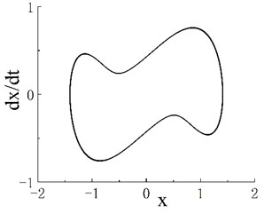
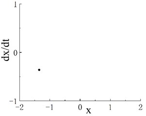
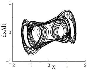
The system performance in response to stable period-1 motion occurs at $0.43 < ω \leq 0.487$ . The phase portrait and Poincaré map when $ω =$ 0.45 are shown in Figs. 2(a1) and 2(a2), respectively. The phase portrait is a universal limit cycle; correspondingly, the Poincaré map exhibits an isolated point. Notably, $0.488 < ω \leq 0.518$ is the first chaotic motion region of the system.

Fig. 1Bifurcation diagram of fractional-order Duffing system with α= 1.2, 0.43<ω≤1.23

$Bifurcation diagram of fractional-order Duffing system with α= 1.2, 0.43<ω≤1.23$

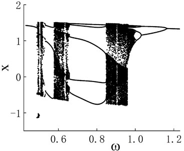
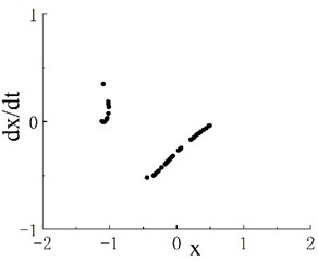
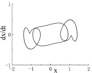
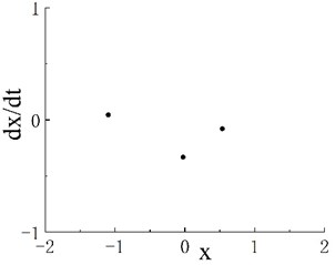
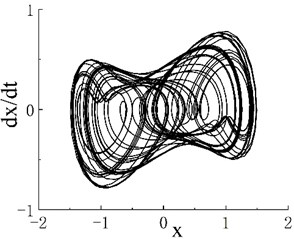
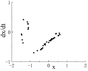
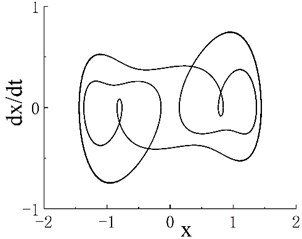
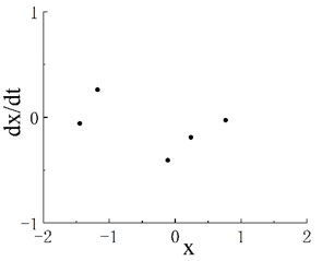
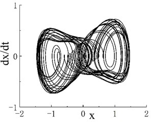
Fig. 2Phase portraits and Poincaré maps of fractional Duffing system. a1) Phase portrait with ω=0.45, a2) Poincaré map with ω=0.45, b1) phase portrait with ω=0.509, b2) Poincaré map with ω=0.509, c1) phase portrait with ω=0.55, c2) Poincaré map with ω=0.55, d1) phase portrait with ω=0.6, d2) Poincaré map with ω=0.6, e1) phase portrait with ω=0.8, e2) Poincaré map with ω=0.8, f1) phase portrait with ω= 0.88, f2) Poincaré map with ω=0.88, g1) phase portrait with ω=1.02 and g2) Poincaré map with ω=1.02

$Phase portraits and Poincaré maps of fractional Duffing system. a1) Phase portrait with ω=0.45, a2) Poincaré map with ω=0.45, b1) phase portrait with ω=0.509, b2) Poincaré map with ω=0.509, c1) phase portrait with ω=0.55, c2) Poincaré map with ω=0.55, d1) phase portrait with ω=0.6, d2) Poincaré map with ω=0.6, e1) phase portrait with ω=0.8, e2) Poincaré map with ω=0.8, f1) phase portrait with ω= 0.88, f2) Poincaré map with ω=0.88, g1) phase portrait with ω=1.02 and g2) Poincaré map with ω=1.02$

a1)

$Phase portraits and Poincaré maps of fractional Duffing system. a1) Phase portrait with ω=0.45, a2) Poincaré map with ω=0.45, b1) phase portrait with ω=0.509, b2) Poincaré map with ω=0.509, c1) phase portrait with ω=0.55, c2) Poincaré map with ω=0.55, d1) phase portrait with ω=0.6, d2) Poincaré map with ω=0.6, e1) phase portrait with ω=0.8, e2) Poincaré map with ω=0.8, f1) phase portrait with ω= 0.88, f2) Poincaré map with ω=0.88, g1) phase portrait with ω=1.02 and g2) Poincaré map with ω=1.02$

a2)

$Phase portraits and Poincaré maps of fractional Duffing system. a1) Phase portrait with ω=0.45, a2) Poincaré map with ω=0.45, b1) phase portrait with ω=0.509, b2) Poincaré map with ω=0.509, c1) phase portrait with ω=0.55, c2) Poincaré map with ω=0.55, d1) phase portrait with ω=0.6, d2) Poincaré map with ω=0.6, e1) phase portrait with ω=0.8, e2) Poincaré map with ω=0.8, f1) phase portrait with ω= 0.88, f2) Poincaré map with ω=0.88, g1) phase portrait with ω=1.02 and g2) Poincaré map with ω=1.02$

b1)

$Phase portraits and Poincaré maps of fractional Duffing system. a1) Phase portrait with ω=0.45, a2) Poincaré map with ω=0.45, b1) phase portrait with ω=0.509, b2) Poincaré map with ω=0.509, c1) phase portrait with ω=0.55, c2) Poincaré map with ω=0.55, d1) phase portrait with ω=0.6, d2) Poincaré map with ω=0.6, e1) phase portrait with ω=0.8, e2) Poincaré map with ω=0.8, f1) phase portrait with ω= 0.88, f2) Poincaré map with ω=0.88, g1) phase portrait with ω=1.02 and g2) Poincaré map with ω=1.02$

b2)

$Phase portraits and Poincaré maps of fractional Duffing system. a1) Phase portrait with ω=0.45, a2) Poincaré map with ω=0.45, b1) phase portrait with ω=0.509, b2) Poincaré map with ω=0.509, c1) phase portrait with ω=0.55, c2) Poincaré map with ω=0.55, d1) phase portrait with ω=0.6, d2) Poincaré map with ω=0.6, e1) phase portrait with ω=0.8, e2) Poincaré map with ω=0.8, f1) phase portrait with ω= 0.88, f2) Poincaré map with ω=0.88, g1) phase portrait with ω=1.02 and g2) Poincaré map with ω=1.02$

c1)

$Phase portraits and Poincaré maps of fractional Duffing system. a1) Phase portrait with ω=0.45, a2) Poincaré map with ω=0.45, b1) phase portrait with ω=0.509, b2) Poincaré map with ω=0.509, c1) phase portrait with ω=0.55, c2) Poincaré map with ω=0.55, d1) phase portrait with ω=0.6, d2) Poincaré map with ω=0.6, e1) phase portrait with ω=0.8, e2) Poincaré map with ω=0.8, f1) phase portrait with ω= 0.88, f2) Poincaré map with ω=0.88, g1) phase portrait with ω=1.02 and g2) Poincaré map with ω=1.02$

c2)

$Phase portraits and Poincaré maps of fractional Duffing system. a1) Phase portrait with ω=0.45, a2) Poincaré map with ω=0.45, b1) phase portrait with ω=0.509, b2) Poincaré map with ω=0.509, c1) phase portrait with ω=0.55, c2) Poincaré map with ω=0.55, d1) phase portrait with ω=0.6, d2) Poincaré map with ω=0.6, e1) phase portrait with ω=0.8, e2) Poincaré map with ω=0.8, f1) phase portrait with ω= 0.88, f2) Poincaré map with ω=0.88, g1) phase portrait with ω=1.02 and g2) Poincaré map with ω=1.02$

d1)

$Phase portraits and Poincaré maps of fractional Duffing system. a1) Phase portrait with ω=0.45, a2) Poincaré map with ω=0.45, b1) phase portrait with ω=0.509, b2) Poincaré map with ω=0.509, c1) phase portrait with ω=0.55, c2) Poincaré map with ω=0.55, d1) phase portrait with ω=0.6, d2) Poincaré map with ω=0.6, e1) phase portrait with ω=0.8, e2) Poincaré map with ω=0.8, f1) phase portrait with ω= 0.88, f2) Poincaré map with ω=0.88, g1) phase portrait with ω=1.02 and g2) Poincaré map with ω=1.02$

d2)

$Phase portraits and Poincaré maps of fractional Duffing system. a1) Phase portrait with ω=0.45, a2) Poincaré map with ω=0.45, b1) phase portrait with ω=0.509, b2) Poincaré map with ω=0.509, c1) phase portrait with ω=0.55, c2) Poincaré map with ω=0.55, d1) phase portrait with ω=0.6, d2) Poincaré map with ω=0.6, e1) phase portrait with ω=0.8, e2) Poincaré map with ω=0.8, f1) phase portrait with ω= 0.88, f2) Poincaré map with ω=0.88, g1) phase portrait with ω=1.02 and g2) Poincaré map with ω=1.02$

e1)

$Phase portraits and Poincaré maps of fractional Duffing system. a1) Phase portrait with ω=0.45, a2) Poincaré map with ω=0.45, b1) phase portrait with ω=0.509, b2) Poincaré map with ω=0.509, c1) phase portrait with ω=0.55, c2) Poincaré map with ω=0.55, d1) phase portrait with ω=0.6, d2) Poincaré map with ω=0.6, e1) phase portrait with ω=0.8, e2) Poincaré map with ω=0.8, f1) phase portrait with ω= 0.88, f2) Poincaré map with ω=0.88, g1) phase portrait with ω=1.02 and g2) Poincaré map with ω=1.02$

e2)

$Phase portraits and Poincaré maps of fractional Duffing system. a1) Phase portrait with ω=0.45, a2) Poincaré map with ω=0.45, b1) phase portrait with ω=0.509, b2) Poincaré map with ω=0.509, c1) phase portrait with ω=0.55, c2) Poincaré map with ω=0.55, d1) phase portrait with ω=0.6, d2) Poincaré map with ω=0.6, e1) phase portrait with ω=0.8, e2) Poincaré map with ω=0.8, f1) phase portrait with ω= 0.88, f2) Poincaré map with ω=0.88, g1) phase portrait with ω=1.02 and g2) Poincaré map with ω=1.02$

f1)

$Phase portraits and Poincaré maps of fractional Duffing system. a1) Phase portrait with ω=0.45, a2) Poincaré map with ω=0.45, b1) phase portrait with ω=0.509, b2) Poincaré map with ω=0.509, c1) phase portrait with ω=0.55, c2) Poincaré map with ω=0.55, d1) phase portrait with ω=0.6, d2) Poincaré map with ω=0.6, e1) phase portrait with ω=0.8, e2) Poincaré map with ω=0.8, f1) phase portrait with ω= 0.88, f2) Poincaré map with ω=0.88, g1) phase portrait with ω=1.02 and g2) Poincaré map with ω=1.02$

f2)

$Phase portraits and Poincaré maps of fractional Duffing system. a1) Phase portrait with ω=0.45, a2) Poincaré map with ω=0.45, b1) phase portrait with ω=0.509, b2) Poincaré map with ω=0.509, c1) phase portrait with ω=0.55, c2) Poincaré map with ω=0.55, d1) phase portrait with ω=0.6, d2) Poincaré map with ω=0.6, e1) phase portrait with ω=0.8, e2) Poincaré map with ω=0.8, f1) phase portrait with ω= 0.88, f2) Poincaré map with ω=0.88, g1) phase portrait with ω=1.02 and g2) Poincaré map with ω=1.02$

g1)

$Phase portraits and Poincaré maps of fractional Duffing system. a1) Phase portrait with ω=0.45, a2) Poincaré map with ω=0.45, b1) phase portrait with ω=0.509, b2) Poincaré map with ω=0.509, c1) phase portrait with ω=0.55, c2) Poincaré map with ω=0.55, d1) phase portrait with ω=0.6, d2) Poincaré map with ω=0.6, e1) phase portrait with ω=0.8, e2) Poincaré map with ω=0.8, f1) phase portrait with ω= 0.88, f2) Poincaré map with ω=0.88, g1) phase portrait with ω=1.02 and g2) Poincaré map with ω=1.02$

g2)

The phase portrait and Poincaré map when $ω = 0.509$ are shown in Figs. 2(b1) and 2(b2), respectively. On the Poincaré map, many discrete points are concentrated in two areas. With the increase in excitation frequency $ω$ , the system enters the period-3 motion region, and its frequency range is $0.519 \leq ω \leq 0.577$ . The phase portrait and Poincaré map when $ω =$ 0.55 are shown in Figs. 2(c1) and 2(c2), respectively. The Poincaré map appears as three isolated points, and $0.578 \leq ω \leq 0.657$ is the second chaotic region of the system. The phase portrait when $ω =$ 0.6 is shown as Fig. 2(d1), and scattered points can be seen on the corresponding Poincaré map in Fig. 2(d2). When $ω \geq 0.658$ , the system enters a stable period-5 motion region, and its interval is $0.658 \leq ω \leq 0.848$ . The phase portrait and Poincaré map when $ω =$ 0.8 are shown in Figs. 2(e1) and 2(e2), respectively. The Poincaré map has five scattered points, and $0.849 \leq ω \leq 0.995$ is the third chaotic motion region. Fig. 2(f1) shows the phase portrait when $ω =$ 0.88, and the corresponding Poincaré map is given in Fig. 2(f2). As $ω$ further increases, the system enters periodic motion from chaotic motion. Fig. 1 indicates that when $ω \geq$ 1.17, the system moves stably in period 1. A period-doubling bifurcation transition region exists between the periodic motion region and the third chaotic motion region. The phase portrait and Poincaré map of the transition region when $ω =$ 1.02 are shown in Figs. 2(g1) and 2(g2), respectively.

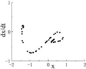
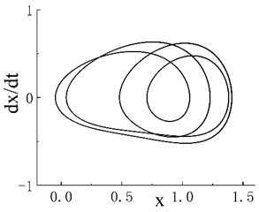
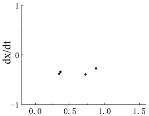
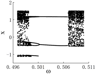
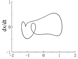
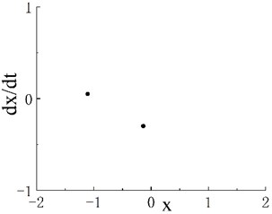
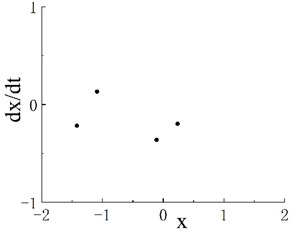
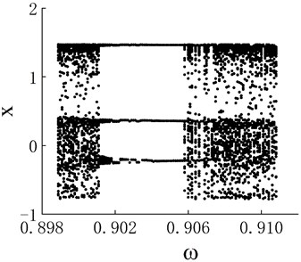
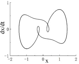
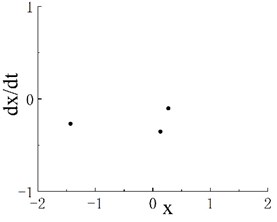
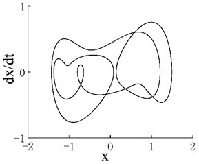
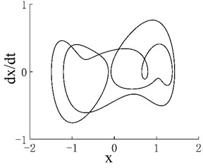
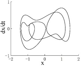
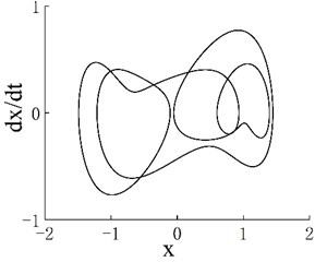
Notably, periodic motion windows are present in the three chaotic motion regions. The bifurcation diagram of the periodic motion window in the first chaotic motion region is shown in Fig. 3(a). The chaotic motion transits from period-doubling motion to period-2 motion. The phase portrait and Poincaré map when $ω =$ 0.506 in the period window are shown in Figs. 3(b) and 3(c), respectively. The bifurcation diagram of the periodic motion window in the second chaotic motion region is shown in Fig. 4(a). In the period window, $ω =$ 0.635 is period-4 motion, and its phase portrait and Poincaré map are shown in Figs. 3(b) and 3(c), respectively. Fig. 5(a) presents the bifurcation diagram of the periodic window in the third chaotic region. Figs. 5(b) and 5(c) respectively show the phase portrait and corresponding Poincaré map when $ω =$ 0.904 in the window.

Fig. 3a) Bifurcation diagram of periodic window in chaotic motion region 1, b) phase portrait when ω= 0.506 and c) Poincaré map when ω= 0.506

a)

b)

c)

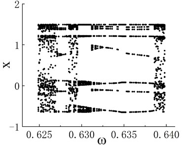
Fig. 4a) Bifurcation diagram of periodic window in chaotic motion region 2, b) phase portrait when ω= 0.635 and c) Poincaré map when ω= 0.635

a)

b)

c)

Fig. 5a) Bifurcation diagram of periodic window in chaotic motion region 3, b) phase portrait when ω= 0.904 and c) Poincaré map when ω= 0.904

a)

b)

c)

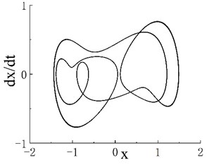
Notably, an interesting change occurs in the periodic window of the second chaotic motion region. Although the system moves in period 4 of the window, the bifurcation diagram has eight dotted lines instead of four solid lines. Although the system exhibits period-4 motion in the period window, the bifurcation diagram has eight dotted lines instead of four solid lines. This observation shows that the motion of the system jumps with the change in frequency in the period window, but it is still period-4 motion. For example, the phase portraits when $ω =$ 0.6352 and $ω =$ 0.6353 are shown in Figs. 6(a) and 6(b), respectively. The phase portraits of two adjacent frequency points are rotated by exactly 180 degrees. When the frequency is further refined, this jumping property remains. Figs. 6(c) and 6(d) present phase portraits with $ω$ of 0.63280 and 0.63281, respectively.

Fig. 6a) Phase portrait with ω= 0.6352, b) phase portrait with ω= 0.6353, c) phase portrait with ω= 0.63280 and d) phase portrait with ω= 0.63281

a)

b)

c)

d)

3.2. Fractional order duffing system with fractional order $α$ or excitation amplitude $f$ fluctuations

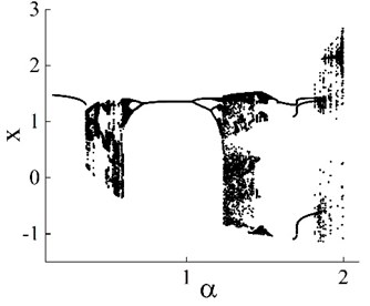
This paper also examines the dynamic characteristics of the system when the fractional order changes. The excitation amplitude is $f =$ 1, the excitation frequency is $ω =$ 1, the basic step length is $h =$ 0.001, the basic truncation term is $N t =$ 10,000, and the step length magnification is $m =$ 5. its memory weakens as the fractional order increases. Thus, the number of truncated items $N_{t}$ is set to decrease by 1000 items with each increase in $α$ by 0.2. The bifurcation diagram is shown in Fig. 7(a). In the process of changing fractional order $α$ from 0.2 to 2, three periodic and three chaotic motion regions appear. The transition is from the first chaotic zone to a stable period-1 motion region after period-doubling bifurcation. As $α$ continues to increase, it enters the second chaotic motion region through period-doubling bifurcation.

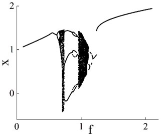
Fig. 7(b) presents the bifurcation diagram of the system when excitation amplitude $f$ fluctuates from 0.1 to 2.1. The fractional order is $α =$ 0.8, the excitation frequency is $ω =$ 1, the basic step length is $h =$ 0.001, the basic truncation item number is $N t =$ 10,000, and the step length magnification is $m =$ 5. The figure shows that three periodic and two chaotic motion regions appear during the fluctuation of excitation amplitude. The first is a stable period-1 motion; the first chaotic motion region is entered through period-doubling bifurcation, followed by entrance to the period-3 motion region. A part of the period-6 movement is contained in the period-3 motion region, and the second chaotic motion region is entered from period-3 motion. As the excitation amplitude continues to increase, the system transitions from the second chaotic region to the period-1 motion region through the period-doubling bifurcation.

Fig. 7a) Bifurcation diagram of x versus α, 0.2<α<2 and b) bifurcation diagram of x versus f, 0.1<f<2.1

a)

b)

4. Conclusions

An improved short memory principle method is introduced to solve the fractional Duffing system numerically. And based on high computational efficiency, some previously unobserved phenomena are obtained. The influence of excitation frequency on the dynamic performance of the system is studied using nonlinear dynamic analysis methods, such as phase portrait, Poincaré map and bifurcation diagram. The bifurcation diagram has four periodic and three chaotic motion regions. The third chaotic motion region exhibits an obvious transition from period-doubling motion to stable period-1 motion. In addition, periodic motion windows are found in the three chaotic motion regions. The periodic motion of the periodic window in the second chaotic motion region has a jumping property. The influence of excitation amplitude and fractional order on the dynamic system performance is also studied. The results show that a change in the system parameters of the fractional Duffing equation affects the dynamic system performance. Thus, such a change shall be considered during the dynamic system design and analysis.

References

K. B. Oldham and J. Spanier, The Fractional Calculus: Theory and Applications of Differentiation and Integration to Arbitrary Order. Dover Publications, 1974.

Search CrossRef
Cannon J. W. and Mandelbrot B. B., “The Fractal Geometry of Nature,” The American Mathematical Monthly, 1984.

Publisher
R. L. Bagley and P. J. Torvik, “Fractional calculus in the transient analysis of viscoelastically damped structures,” AIAA Journal, Vol. 23, No. 6, pp. 918–925, Jun. 1985, https://doi.org/10.2514/3.9007

Publisher
R. L. Bagley and P. J. Torvik, “Fractional calculus – A different approach to the analysis of viscoelastically damped structures,” AIAA Journal, Vol. 21, No. 5, pp. 741–748, May 1983, https://doi.org/10.2514/3.8142

Publisher
Y. Yu, H.-X. Li, S. Wang, and J. Yu, “Dynamic analysis of a fractional-order Lorenz chaotic system,” Chaos, Solitons and Fractals, Vol. 42, No. 2, pp. 1181–1189, Oct. 2009, https://doi.org/10.1016/j.chaos.2009.03.016

Publisher
T. T. Hartley, C. F. Lorenzo, and H. Killory Qammer, “Chaos in a fractional order Chua’s system,” IEEE Transactions on Circuits and Systems I: Fundamental Theory and Applications, Vol. 42, No. 8, pp. 485–490, 1995, https://doi.org/10.1109/81.404062

Publisher
O. P. Agrawal, “A general formulation and solution scheme for fractional optimal control problems,” Nonlinear Dynamics, Vol. 38, No. 1-4, pp. 323–337, Dec. 2004, https://doi.org/10.1007/s11071-004-3764-6

Publisher
Y. Chen, B. M. Vinagre, and I. Podlubny, “Continued fraction expansion approaches to discretizing fractional order derivatives – an expository review,” Nonlinear Dynamics, Vol. 38, No. 1-4, pp. 155–170, Dec. 2004, https://doi.org/10.1007/s11071-004-3752-x

Publisher
S. Jiménez, J. A. González, and L. Vázquez, “Fractional Duffing’s equation and geometrical resonance,” International Journal of Bifurcation and Chaos, Vol. 23, No. 5, p. 1350089, May 2013, https://doi.org/10.1142/s0218127413500892

Publisher
J.-H. Jia, X.-Y. Shen, and H.-X. Hua, “Viscoelastic behavior analysis and application of the fractional derivative maxwell model,” Journal of Vibration and Control, Vol. 13, No. 4, pp. 385–401, Apr. 2007, https://doi.org/10.1177/1077546307076284

Publisher
A. Shokooh and L. Suárez, “A comparison of numerical methods applied to a fractional model of damping materials,” Journal of Vibration and Control, Vol. 5, No. 3, pp. 331–354, May 1999, https://doi.org/10.1177/107754639900500301

Publisher
R. S. Barbosa and J. A. T. Machado, “Describing function analysis of systems with impacts and backlash,” Nonlinear Dynamics, Vol. 29, No. 1/4, pp. 235–250, 2002, https://doi.org/10.1023/a:1016514000260

Publisher
W. Zhang, S. Zhou, H. Li, and H. Zhu, “Chaos in a fractional-order Rössler system,” Chaos, Solitons and Fractals, Vol. 42, No. 3, pp. 1684–1691, Nov. 2009, https://doi.org/10.1016/j.chaos.2009.03.069

Publisher
J. A. T. Machado, D. Baleanu, W. Chen, and J. Sabatier, “New trends in fractional dynamics,” Journal of Vibration and Control, Vol. 20, No. 7, pp. 963–963, May 2014, https://doi.org/10.1177/1077546313507652

Publisher
X. Li and R. Wu, “Hopf bifurcation analysis of a new commensurate fractional-order hyperchaotic system,” Nonlinear Dynamics, Vol. 78, No. 1, pp. 279–288, Oct. 2014, https://doi.org/10.1007/s11071-014-1439-5

Publisher
D. Chen, C. Wu, H. H. C. Iu, and X. Ma, “Circuit simulation for synchronization of a fractional-order and integer-order chaotic system,” Nonlinear Dynamics, Vol. 73, No. 3, pp. 1671–1686, Aug. 2013, https://doi.org/10.1007/s11071-013-0894-8

Publisher
Y.-J. Shen, P. Wei, and S.-P. Yang, “Primary resonance of fractional-order van der Pol oscillator,” Nonlinear Dynamics, Vol. 77, No. 4, pp. 1629–1642, Sep. 2014, https://doi.org/10.1007/s11071-014-1405-2

Publisher
N. Srinil and H. Zanganeh, “Modelling of coupled cross-flow/in-line vortex-induced vibrations using double Duffing and van der Pol oscillators,” Ocean Engineering, Vol. 53, pp. 83–97, Oct. 2012, https://doi.org/10.1016/j.oceaneng.2012.06.025

Publisher
P. Brzeski, P. Perlikowski, and T. Kapitaniak, “Numerical optimization of tuned mass absorbers attached to strongly nonlinear Duffing oscillator,” Communications in Nonlinear Science and Numerical Simulation, Vol. 19, No. 1, pp. 298–310, Jan. 2014, https://doi.org/10.1016/j.cnsns.2013.06.001

Publisher
N. M. M. Maia, J. M. M. Silva, and A. M. R. Ribeiro, “On a general model for damping,” Journal of Sound and Vibration, Vol. 218, No. 5, pp. 749–767, Dec. 1998, https://doi.org/10.1006/jsvi.1998.1863

Publisher
T. T. Hartley and C. F. Lorenzo, “A frequency-domain approach to optimal fractional-order damping,” Nonlinear Dynamics, Vol. 38, No. 1-4, pp. 69–84, Dec. 2004, https://doi.org/10.1007/s11071-004-3747-7

Publisher
Y. Wang and J.-Y. An, “Amplitude-frequency relationship to a fractional Duffing oscillator arising in microphysics and tsunami motion,” Journal of Low Frequency Noise, Vibration and Active Control, Vol. 38, No. 3-4, pp. 1008–1012, Dec. 2019, https://doi.org/10.1177/1461348418795813

Publisher
Z. Li, D. Chen, J. Zhu, and Y. Liu, “Nonlinear dynamics of fractional order Duffing system,” Chaos, Solitons and Fractals, Vol. 81, pp. 111–116, Dec. 2015, https://doi.org/10.1016/j.chaos.2015.09.012

Publisher
Duan Junsheng, Sun Jie, and Temuer Chaolu, “Nonlinear fractional differential equation combining duffing equation and van der pol equation,” Shuxue Zazhi, Vol. 31, No. 1, pp. 7–10, 2011.

Search CrossRef
J. Niu, R. Liu, Y. Shen, and S. Yang, “Chaos detection of Duffing system with fractional-order derivative by Melnikov method,” Chaos: An Interdisciplinary Journal of Nonlinear Science, Vol. 29, No. 12, p. 123106, Dec. 2019, https://doi.org/10.1063/1.5124367

Publisher
R. Wang, H. Zhang, and Y. Zhang, “Bifurcation and vibration resonance in the time delay Duffing system with fractional internal and external damping,” Meccanica, Vol. 57, No. 5, pp. 999–1015, May 2022, https://doi.org/10.1007/s11012-022-01483-y

Publisher
A. Ouannas, A.-A. Khennaoui, S. Momani, and V.-T. Pham, “The discrete fractional duffing system: Chaos, 0-1 test, C₀ complexity, entropy, and control,” Chaos: An Interdisciplinary Journal of Nonlinear Science, Vol. 30, No. 8, p. 083131, Aug. 2020, https://doi.org/10.1063/5.0005059

Publisher

Cited by

Implicit Finite-Difference Scheme for a Duffing Oscillator with a Derivative of Variable Fractional Order of the Riemann-Liouville Type

Valentine Aleksandrovich Kim | Roman Ivanovich Parovik | Zafar Ravshanovich Rakhmonov

(2023)

About this article

Received

29 September 2021

Accepted

29 April 2022

Published

23 August 2022

SUBJECTS

Chaos, nonlinear dynamics and applications

DOI

https://doi.org/10.21595/jve.2022.22230

Keywords

fractional calculus

bifurcation

chaos

short memory principle

Acknowledgements

This work was supported by the National Natural Science Foundation of China [Grant No. 11472133].

This is an open access article distributed under the Creative Commons Attribution License, which permits unrestricted use, distribution, and reproduction in any medium, provided the original work is properly cited.

Previous article in issue Previous Next article in issue Next

Research article

2019 05 15

Stochastic P-bifurcation in a tri-stable Van der Pol system with fractional derivative under Gaussian white noise

Yajie Li, Zhiqiang Wu

Research article

2018 06 30

Bifurcation and chaos analysis of a gear pair system with multi-clearance

Yan Xia, Yi Wan, Xichang Liang

Research article

2018 02 15

Dynamical response of fractional-order nonlinear system with combined parametric and forcing excitation

Hai Jun Xing, Ke Shi Xiao, Peng Sai Song, Lin Ru Li

Research article

2017 03 31

Bursting oscillation and bifurcation mechanism in fractional-order Brusselator with two different time scales

Jufeng Chen, Xianghong Li, Jingyu Hou, Dawei Zuo

R. Ma, B. Zhang, and J. Han, “Bifurcation analysis of fractional duffing system based on improved short memory principle method,” Journal of Vibroengineering, Vol. 24, No. 6, pp. 1162–1173, Aug. 2022, https://doi.org/10.21595/jve.2022.22230

Copy Extrica

Copied to clipboard!

TY  - JOUR
DO  - 10.21595/jve.2022.22230
UR  - https://doi.org/10.21595/jve.2022.22230
TI  - Bifurcation analysis of fractional duffing system based on improved short memory principle method
T2  - Journal of Vibroengineering
AU  - Ma, Ruiqun
AU  - Zhang, Bo
AU  - Han, Jinglong
PY  - 2022
DA  - 2022/08/23
PB  - JVE International Ltd.
SP  - 1162-1173
VL  - 24
IS  - 6
SN  - 1392-8716
SN  - 2538-8460
ER  - 

Copy Ris

Copied to clipboard!

@article{Ma_2022,
	doi = {10.21595/jve.2022.22230},
	url = {https://doi.org/10.21595/jve.2022.22230},
	year = 2022,
	month = {aug},
	publisher = {{JVE} International Ltd.},
	volume = {24},
	number = {6},
	pages = {1162--1173},
	author = {Ruiqun Ma and Bo Zhang and Jinglong Han},
	title = {Bifurcation analysis of fractional duffing system based on improved short memory principle method},
	journal = {Journal of Vibroengineering}
}

Copy Bibtex

Copied to clipboard!

[1]R. Ma, B. Zhang, and J. Han, “Bifurcation analysis of fractional duffing system based on improved short memory principle method,” Journal of Vibroengineering, vol. 24, no. 6, pp. 1162–1173, Aug. 2022, doi: 10.21595/jve.2022.22230.

Copy IEEE

Copied to clipboard!

Ma, Ruiqun, Bo Zhang, and Jinglong Han. “Bifurcation Analysis of Fractional Duffing System Based on Improved Short Memory Principle Method.” Journal of Vibroengineering 24, no. 6 (August 23, 2022): 1162–73. https://doi.org/10.21595/jve.2022.22230.

Copy Chicago

Copied to clipboard!

Bifurcation analysis of fractional duffing system based on improved short memory principle method

Abstract

1. Introduction

2. Fractional duffing system

2.1. Fractional differential definition

2.2. Improved short memory principle method

2.3. Basis for step enlargement

2.4. Fractional duffing system

3. Nonlinear dynamic analysis of fractional duffing system

3.1. Fractional order duffing system with α=1.2 and f=0.6

3.2. Fractional order duffing system with fractional order α or excitation amplitude f fluctuations

4. Conclusions

References

Cited by

About this article

Related Articles

3.1. Fractional order duffing system with $α = 1.2$ and $f = 0.6$

3.2. Fractional order duffing system with fractional order $α$ or excitation amplitude $f$ fluctuations