Vertical vibration modeling for 2:1-roping traction elevator system

Shi, Jipeng; Zhang, Weimin; Wu, Chengjun

doi:10.21595/jve.2021.22243

Journal of Vibroengineering

Browse Journal

Submit article

Published: 17 March 2022

Check for updates

Vertical vibration modeling for 2:1-roping traction elevator system

Jipeng Shi¹

Weimin Zhang²

Chengjun Wu³

^{1, 2, 3}School of Mechanical Engineering, Xi’an Jiaotong University, Xi’an, Shaanxi, 710049, China

Corresponding Author:

Chengjun Wu

Cite the article Download PDF

Downloads 664

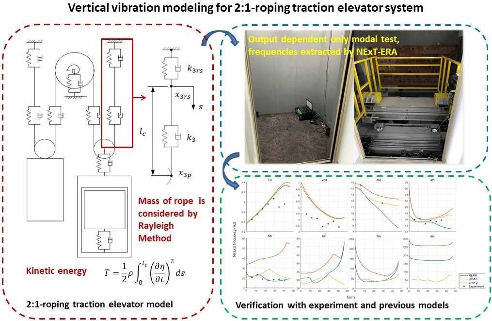
Abstract

This paper presents a vertical vibration model for 2:1-roping traction elevator system. In this model, masses of suspension ropes are considered and their kinetic energy is calculated by applying Rayleigh method. Equations of motion for free vibration are derived. To verify the improvement of the model, an output dependent only modal test scheme using eigenvalue realization algorithm is conducted to obtain natural frequencies from a real elevator installation. The comparison of experimental results and numerical results of proposed model and previous similar models is presented on calculation of natural frequencies. The results show that proposed model is able to reflect the 5th natural frequencies more exactly under 0 % and 100 % load conditions.

Vertical vibration modeling for 2:1-roping traction elevator system

Highlights

A vertical elevator model considering masses of suspension ropes by Rayleigh method is proposed
Output dependent only modal test using NExT-ERA is designed and conducted
The proposed model calculates the 5th order natural frequency more accurate than similar models

1. Introduction

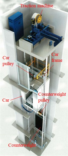
The traction elevator installation is a system that contains large mass components and connected by necessary flexible components, a universal 2:1-roping configuration (rope twine once around a pulley on car-side or counterweight-side) is shown as Fig. 1. To help understand elevator’s vertical dynamic property thereby improve the product’s performance, various simplified models have been proposed by researchers.

Fig. 1Basic structure of 2:1-roping elevator

To investigate the elevator from a scope of the entire system, commonly approach is to lump the masses at several discrete points and then the model formed has limited degree of freedoms (DOFs), which is called lumped parameter model (LPM) [1]. Depending on the structure of the installation and how much detail is concerned, models with different DOFs are proposed. So far, there have been a lot of successful applications of LPM on both 1:1- and 2:1-roping configurations, such as analysis of dynamic characteristics of the entire system [2], [3], the design of status observer and vibration controller [4]-[6] and parameter optimization [7], the number of DOF of the model ranges from 5 [2] to 27 [8]. In previous studies using LPM, some have taken into account the masses of the suspension ropes, the approach of treating the masses of ropes is also lumping them into several mass points, the more the mass points, the more accurate intrinsic characteristics can be captured.

It is not hard to imagine that when the suspension ropes are regarded as a continuum, the system characteristics will be described more accurately, leading to model with infinitive DOFs which known as distributed parameter model (DPM) [1]. Continuous treatment can be multi-dimensional, that means not only the multi-dimensional DPM includes vertical direction, but also horizontal directions. Various phenomena had been investigated using DPMs, such as the vertical vibration caused by drive system [9], the passage through resonance [10], [11], the coupled vibration of elevator and building [12] and the interaction between elevator components and building [13]. Researches on DPM for engineering purposes are relatively fewer, for instance the vibration controller design [14].

In terms of the applicability of these two types of model in the study of vertical features of elevator system, Arrasate et al. [1] compared a 5-DOF 1:1-roping LPM with a corresponding DPM. The results showed that LPM is as accurate as DPM for the first few orders (the first three orders for natural frequencies and the first four orders for mode shapes), LPM had also been proved to be precise enough for response prediction of the car because only the first few orders contribute largely to total vibration. This study reveals that compared with LPM, DPM does not show great superior in depicting dynamic characteristics mainly determined by large-mass components in traction elevator system. Besides, it can be seen from previous studies, the application of LPM is more diversified since this type of model has the convenience for modeling and is easy to be popularized to more complex situations. By contrast, modeling and solving of DPM for an entire elevator system can be cumbersome, which brings difficulties to further design based on the model. Based on the above reasons, LPM is focused in this paper.

As mentioned, in the use of LPM, masses of suspension ropes are generally ignored or modeled as lumped mass points, which is not so close to the physical properties. It is known from Rayleigh method, a proper equivalence of distributed mass of ropes in calculating the kinetic energy will lead to a good approximation of natural frequencies (NFs), which probably help improve the accuracy of current LPMs. In this paper, a vertical vibration model for 2:1-roping elevator system with 8 DOFs is developed. Then the equations of motion are derived by applying Rayleigh method in the calculation of kinetic energy. Next, a feasible modal test procedure is designed to obtain NFs of a real elevator installation. Finally, the effectiveness and improvement of proposed model is verified by experimental results and numerical results calculated from conventional LPMs without and with the masses of ropes.

2. Vertical vibration model

In this section, a vertical vibration model for 2:1-roping elevator system is introduced and equations of motion of the model are derived.

2.1. Model description

Consider the main components shown in Fig. 1, 8-DOF model can be established, see Fig. 2.

In model shown in Fig. 2, multiple components in the actual structure are regarded as one object, such as car pulleys, suspension ropes, rubber cushions and rope-end spring combinations. $x_{1} ~ x_{5}$ donate the translational displacements of car, car frame, car pulley, traction sheave and counterweight pulley, respectively. $θ_{3} ~ θ_{5}$ donate the rotational displacements of the car pulley, traction sheave and counterweight pulley. Suppose every displacement coordinate has its origin on the static equilibrium position. The traction sheave is directly installed on the main body of traction machine thus they share the same translational DOF with displacement $x_{4}$ . In the same way, counterweight pulley and counterweight block also share the same translational DOF with displacement $x_{5}$ .

$m_{1}$ donates the total mass of car and actual load. $m_{2}$ donates the total mass of car frame and car-side compensation chain which is time-variant. $m_{3}$ donates the total mass of car pulley and peripheral supporting structures. $m_{4}$ is the mass of traction machine (including sheave and main body). $m_{5}$ is the mass of counterweight (including pulley and block) and counterweight-side compensation chain. $J_{3}$ and $R_{c}$ are inertia moment and radius of car pulley, $J_{4}$ , $R_{c}$ and $J_{5}$ , $R_{w}$ are the corresponding parameters of traction sheave and counterweight pulley. Noting that value of each inertia moment is computed by the mass of pulley or sheave only.

Fig. 2Vertical vibration model of 2:1-ropping elevator

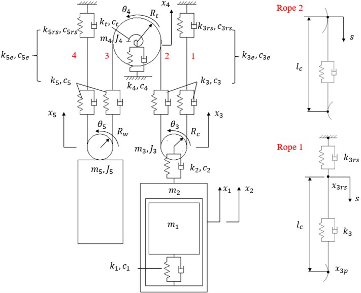
All the flexible connections are modeled as parallel ideal springs and viscous dampers. The elasticity compensation chain between car frame and counterweight is omitted in Fig. 2. $k_{1}$ , $k_{2}$ and $k_{4}$ represent stiff coefficients of cushions installed in corresponding positions. $k_{t}$ is the rotational stiffness of traction sheave. An intact suspension rope that winds through car pulley, traction sheave and counterweight pulley is divided into four isolate pieces without considering the short parts that lay on wheel grooves, namely rope 1~4. Every end of a piece of rope is consolidated with adjacent component. Suppose rope 1 and 2 have the same length $l_{c}$ and rope 3 and 4 have the same length $l_{w}$ . $k_{3}$ is the stiff coefficient of rope 1 or 2, $k_{5}$ is the stiff coefficient of rope 3 or 4, $k_{3 r s}$ and $k_{5 r s}$ are stiff coefficients of car-side and counterweight-side rope-end springs. Symbol $c$ with same subscript as $k$ represents corresponding parallel damping coefficient.

2.2. Equations of motion

The ropes are considered as springs with masses. Follow the idea of Rayleigh method, the displacement function of the rope should be given firstly to calculate the kinetic energy. Take rope 2 as example, the displacement function of rope 2 can be assumed as:

1

η (s, t) = B_{1} s + B_{2},

where multipliers $B_{1}$ and $B_{2}$ are determined by the following boundary conditions:

2

{η (s, t) |}_{s = 0} = x_{4} + R_{t} θ_{4}, {η (s, t) |}_{s = l_{c}} = x_{3} - R_{c} θ_{3},

substituting Eq. (2) in Eq. (1) yields:

3

B_{1} = \frac{(x_{3} - R_{c} θ_{3}) - (x_{4} + R_{t} θ_{4})}{l_{c}}, B_{2} = x_{4} + R_{t} θ_{4} .

The mass of rope depends on its length, which is given by $m_{r c / r w} = ρ l_{c / w}$ . For a certain integral upper limit, the kinetic energy of rope 2 is computed as:

4

T_{r 2} = \frac{1}{2} ρ \int_{0}^{l_{c}} {(\frac{\partial η}{\partial t})}^{2} d s = \frac{1}{2} ρ \int_{0}^{l_{c}} {[(1 - \frac{s}{l_{c}}) ({\dot{x}}_{4} + R_{t} {\dot{θ}}_{4}) + \frac{s}{l_{c}} ({\dot{x}}_{3} - R_{c} {\dot{θ}}_{3})]}^{2} d s

= \frac{1}{6} m_{r c} [{({\dot{x}}_{3} - R_{c} {\dot{θ}}_{3})}^{2} + {({\dot{x}}_{4} + R_{t} {\dot{θ}}_{4})}^{2} + ({\dot{x}}_{3} - R_{c} {\dot{θ}}_{3}) ({\dot{x}}_{4} + R_{t} {\dot{θ}}_{4})] .

Similarly, the kinetic energy of the rope 3 is expressed as:

5

T_{r 3} = \frac{1}{6} m_{r w} [{({\dot{x}}_{5} + R_{w} {\dot{θ}}_{5})}^{2} + {({\dot{x}}_{4} - R_{t} {\dot{θ}}_{4})}^{2} + ({\dot{x}}_{5} + R_{w} {\dot{θ}}_{5}) ({\dot{x}}_{4} - R_{t} {\dot{θ}}_{4})] .

Consider rope 1, for the convenience of illustration, let $x_{3 r s}$ represent the displacement of the junction of rope 1 and rope-end spring, let $x_{3 p}$ represent the displacement of the junction of the rope 1 and car pulley, see Fig. 2. Consequently, Hooke’s law yields:

6

\frac{∆ x_{3 p}}{∆ x_{3 r s}} = \frac{k_{3 r s}}{k_{3}} .

The fixation of upper end of the spring results in:

7

∆ x_{3 r s} = x_{3 r s} .

Additionally, the displacement variation $Δ x_{3 p}$ can be expressed as:

8

∆ x_{3 p} = x_{3 p} - x_{3 r s} .

Therefore, substituting Eq. (8) and Eq. (7) in Eq. (6) yields:

9

x_{3 r s} = \frac{k_{3}}{k_{3} + k_{3 r s}} x_{3 p} .

Also consider the boundary condition:

10

{η (s, t) |}_{s = 0} = x_{3 r s}, {η (s, t) |}_{s = l_{c}} = {x_{3 p} = x}_{3} + R_{c} θ_{3},

the kinetic energy of rope 1 can be obtained by same process:

11

T_{r 1} = \frac{1}{2} ρ \int_{0}^{l_{c}} {(\frac{\partial η}{\partial t})}^{2} d s = \frac{1}{6} m_{r c} [{(\frac{k_{3}}{k_{3} + k_{3 r s}} {\dot{x}}_{3 p})}^{2} + \frac{k_{3}}{k_{3} + k_{3 r s}} {\dot{x}}_{3 p}^{2} + {\dot{x}}_{3 p}^{2}]

= \frac{1}{6} m_{r c} [{(\frac{k_{3}}{k_{3} + k_{3 r s}})}^{2} {({\dot{x}}_{3} + R_{c} {\dot{θ}}_{3})}^{2} + \frac{k_{3}}{k_{3} + k_{3 r s}} {({\dot{x}}_{3} + R_{c} {\dot{θ}}_{3})}^{2} + {({\dot{x}}_{3} + R_{c} {\dot{θ}}_{3})}^{2}]

= \frac{1}{6} m_{r c} k_{3 c o e} {({\dot{x}}_{3} + R_{c} {\dot{θ}}_{3})}^{2},

where $k_{3 c o e}$ is coefficient determined by $k_{3}$ and $k_{3 r s}$ :

12

k_{3 c o e} = 1 + \frac{k_{3}}{k_{3} + k_{3 r s}} + {(\frac{k_{3}}{k_{3} + k_{3 r s}})}^{2} .

The kinetic energy of the rope 4 is:

13

T_{r 4} = \frac{1}{6} m_{r w} k_{5 c o e} {({\dot{x}}_{5} - R_{w} {\dot{θ}}_{5})}^{2},

with:

14

k_{5 c o e} = 1 + \frac{k_{5}}{k_{5} + k_{5 r s}} + {(\frac{k_{5}}{k_{5} + k_{5 r s}})}^{2} .

The stiffness of rope is also length-dependent, stiffness coefficient is given by $k_{3 / 5} = E_{r} A / l_{c / w}$ . When the sizes of the car and counterweight are both neglected and suppose the car moves upward, $l_{c}$ and $l_{w}$ can be computed as follows:

15

l_{c} = H + H_{m i n} - h (t),

16

l_{w} = H_{m i n} + h (t) .

Generally, there are compensation chains linked between car frame and counterweight for the sake of balance, this kind of attached mass should be involved in the car frame and counterweight. Hence, mass $m_{2}$ and $m_{5}$ can be expressed as:

17

m_{2} = m_{f} + ρ_{c p} [H_{m i n c p} + h (t)],

18

m_{5} = m_{w} + ρ_{c p} (H_{e l v} + H_{m i n c p} - l_{w}) .

For various lumped mass parts in model, the translational kinetic energy is $m_{i} {\dot{x}}_{i}^{2} / 2$ ( $i =$ 1, 2, 3, 4, 5) and rotational kinetic energy is $J_{j} {\dot{θ}}_{j}^{2} / 2$ ( $j =$ 3, 4, 5). As a result, the total kinetic energy of the system can be given as:

19

T = \frac{1}{2} \sum_{i = 1}^{5} m_{i} {\dot{x}}_{i}^{2} + \frac{1}{2} \sum_{i = 3}^{5} J_{i} {\dot{θ}}_{i}^{2} + \frac{1}{6} m_{r c} k_{3 c o e} {({\dot{x}}_{3} + R_{c} {\dot{θ}}_{3})}^{2} + \frac{1}{6} m_{r w} k_{5 c o e} {({\dot{x}}_{5} - R_{w} {\dot{θ}}_{5})}^{2}

+ \frac{1}{6} m_{r c} [{({\dot{x}}_{3} - R_{c} {\dot{θ}}_{3})}^{2} + {({\dot{x}}_{4} + R_{t} {\dot{θ}}_{4})}^{2} + ({\dot{x}}_{3} - R_{c} {\dot{θ}}_{3}) ({\dot{x}}_{4} + R_{t} {\dot{θ}}_{4})]

+ \frac{1}{6} m_{r w} [{({\dot{x}}_{5} + R_{w} {\dot{θ}}_{5})}^{2} + {({\dot{x}}_{4} - R_{t} {\dot{θ}}_{4})}^{2} + ({\dot{x}}_{5} + R_{w} {\dot{θ}}_{5}) ({\dot{x}}_{4} - R_{t} {\dot{θ}}_{4})] .

Consider the relative displacement of two ends of all flexible components, the total potential energy is expressed as:

20

U = \frac{1}{2} {k_{1} {(x_{1} - x_{2})}^{2} + k_{2} {(x_{2} - x_{3})}^{2} + k_{4} {x_{4}}^{2} + k_{t} {θ_{4}}^{2}

+ k_{3} {[(x_{3} - R_{c} θ_{3}) - (x_{4} + R_{t} θ_{4})]}^{2} + k_{5} {[(x_{4} - R_{t} θ_{4}) - (x_{5} + R_{w} θ_{5})]}^{2}

+ k_{3 e} {(x_{3} + R_{c} θ_{3})}^{2} + k_{5 e} {(x_{5} - R_{w} θ_{5})}^{2}} .

Owing to the viscous damping assumption is made in this model, the energy dissipation $Ψ$ can be obtained easily from the expression of $U$ by replacing $k$ , $x$ and $θ$ by corresponding $c$ , $\dot{x}$ and $\dot{θ}$ respectively.

Lagrange equation with dissipation term is given by:

21

\frac{d}{d t} (\frac{\partial L}{\partial {\dot{q}}_{k}}) - \frac{\partial L}{\partial q_{k}} - \frac{\partial Ψ}{\partial {\dot{q}}_{k}} = 0,

where $L = T - U$ , $q_{k}$ represents the generalized coordinate. By substituting $T$ , $U$ and $Ψ$ , equations of motion for free vibration can be written as:

22

M \ddot{x} + C \dot{x} + K x = 0,

where:

23

x = {[\begin{matrix} x_{1} & x_{2} & x_{3} & θ_{3} & x_{4} & θ_{4} & x_{5} & θ_{5} \end{matrix}]}^{T},

24

M = [\begin{matrix} m_{1} & 0 & 0 & 0 & 0 \\ m_{2} & 0 & 0 & 0 \\ m_{3} + \frac{1}{3} m_{r c} (1 + k_{3 c o e}) & \frac{1}{3} m_{r c} R_{c} (k_{3 c o e} - 1) & \frac{1}{6} m_{r c} \\ J_{3} + \frac{1}{3} m_{r c} {R_{c}}^{2} (1 + k_{3 c o e}) & - \frac{1}{6} m_{r c} R_{c} \\ m_{4} + \frac{1}{3} (m_{r c} + m_{r w}) \\ S y m m e t r i c \end{matrix}

\begin{matrix} 0 & 0 & 0 \\ 0 & 0 & 0 \\ \frac{1}{6} m_{r c} R_{t} & 0 & 0 \\ - \frac{1}{6} m_{r c} R_{c} R_{t} & 0 & 0 \\ \frac{1}{3} R_{t} (m_{r c} - m_{r w}) & \frac{1}{6} m_{r w} & \frac{1}{6} m_{r w} R_{w} \\ J_{4} + \frac{1}{3} {R_{t}}^{2} (m_{r c} + m_{r w}) & - \frac{1}{6} m_{r w} R_{t} & - \frac{1}{6} m_{r w} {R_{w} R}_{t} \\ m_{5} + \frac{1}{3} m_{r w} (1 + k_{5 c o e}) & \frac{1}{3} m_{r w} R_{w} (1 - k_{5 c o e}) \\ J_{5} + \frac{1}{3} m_{r w} R_{w} (1 + k_{5 c o e}) \end{matrix}],

25

K = [\begin{matrix} k_{1} & - k_{1} & 0 & 0 & 0 \\ k_{1} + k_{2} & - k_{2} & 0 & 0 \\ k_{2} + k_{3} + k_{3 e} & (k_{3 e} - k_{3}) R_{c} & - k_{3} \\ (k_{3} + k_{3 e}) {R_{c}}^{2} & k_{3} R_{c} \\ k_{3} + k_{4} + k_{5} \\ S y m m e t r i c \end{matrix}

\begin{matrix} 0 & 0 & 0 \\ 0 & 0 & 0 \\ - k_{3} R_{t} & 0 & 0 \\ k_{3} R_{c} R_{t} & 0 & 0 \\ (k_{3} - k_{5}) R_{t} & - k_{5} & - k_{5} R_{w} \\ (k_{3} + k_{5}) {R_{t}}^{2} + k_{t} & k_{5} R_{t} & k_{5} {R_{w} R}_{t} \\ k_{5} + k_{5 e} & (k_{5} - k_{5 e}) R_{w} \\ (k_{5} + k_{5 e}) {R_{w}}^{2} \end{matrix}] .

Vector $\ddot{x}$ and $\dot{x}$ are second time derivative and first-time derivative of $x$ . $k_{3 e}$ and $k_{5 e}$ are equivalent stiff coefficients, which are given as $k_{3} k_{3 r s} / (k_{3} + k_{3 r s})$ and $k_{5} k_{5 r s} / (k_{5} + k_{5 r s})$ , respectively. Matrix $C$ has the same form of $K$ with replacing $k$ by corresponding $c$ .

Because of the difficulty in giving elements in $C$ separately and directly, proportional damping matrix is often used instead in a small damping system when two coefficients $α$ and $β$ can be selected properly, which is expressed as:

26

C = α M + β K .

Specifying modal damping ratio $ζ$ is also often adopted in engineering. Therefore, $C$ can be obtained as follow:

27

C = {(Φ^{- 1})}^{T} C_{p} Φ^{- 1} = (M Φ {M_{p}}^{- 1}) C_{p} ({M_{p}}^{- 1} Φ^{T} M) = \sum_{i = 1}^{8} \frac{2 ζ_{i} ω_{i}}{M_{p i}} (M ϕ_{i}) {(M ϕ_{i})}^{T},

where $Φ$ donates the modal matrix determined by the eigenvalue problem related to $M$ and $K$ . Subscript ${()}_{p}$ represents a matrix that has been normalized by $Φ$ .

3. Numerical and experimental verification

To verify the correctness of the model illustrated above, numerical and experimental study are performed on a real elevator installation aiming at obtain NFs of the system. Basic parameters of the installation are given in Table 1. The values in Table 1 have considered the number of components in actual structure. The tested installation has no rope-end spring, for that reason a large number 10¹⁰ is used in calculation to approximate rigid connection.

In numerical computation, undamped NFs are obtained by solving the eigenvalue function $|K - ω^{2} M| = 0$ with $h$ increasing in small steps.

The proposed Rayleigh lumped parameter model will be called “RLPM” in the following content. The corresponding conventional LPMs without and with rope masses, namely “LPM-1” and “LPM-2”, are also participate calculation. In LPM-2, mass points of four pieces of ropes make the number of DOF become 12, for the purposes of comparison, only the first 8 orders are used. The numerical results will be compared together with the experimental results later.

Table 1Key parameters of the tested elevator

Symbol	Value	Unit	Symbol	Value	Unit
$H$	46.5	m	$m_{4 s h}$	37.3	kg
$H_{m i n}$	2.54	m	$m_{5}$	1449.85	kg
$H_{m i n c p}$	1	m	$m_{5 p}$	15	kg
$Q$	1000	kg	$ρ$	1.54	kg/m
$R_{c}$	0.16	m	$ρ_{c p}$	0.974	kg/m
$R_{w}$	0.16	m	$k_{1}$	2.6×10⁶	N/m
$R_{t}$	0.16	m	$k_{2}$	3.3×10⁶	N/m
$m_{c}$	525.21	kg	$k_{4}$	1.3×10⁶	N/m
$m_{f}$	389.34	kg	$k_{t}$	1.2×10⁶	N/m
$m_{3}$	85.3	kg	$E_{r}$	6×10¹⁰	N
$m_{3 p}$	40	kg	$A$	3.5186×10^-4	m^-²
$m_{4}$	265	kg

4. Experimental procedure

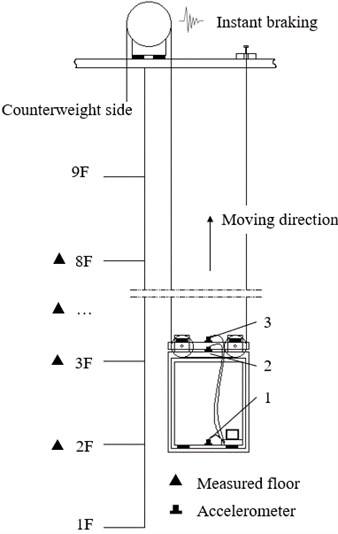
Fig. 3 shows the experimental scheme.

Fig. 3Schematic diagram of experimental scheme

Steps of the test are listed as follows:

1) Arrange test instruments. Three accelerometers (B&K 4535-B-001 with sampling frequency at 1000 Hz) numbered from 1 to 3 are fixed at three locations separately, which are the center of the car’s ground, the top of the car frame and the top of the car pulley beam. Data collector (B&K LAN-XI) and a personal computer (PC) are placed inside the car. Fig. 4 shows the setup on the scene.

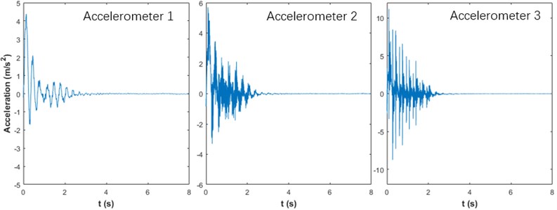
2) Choose the 2nd floor to the 8th floor as measurement positions. Let the car run upward with 0 % load and brake the traction machine instantly when car near each floor, the elevator system will vibrate freely and acceleration responses are measured. A set of collected signals are shown as Fig. 5.

Fig. 4Experimental setup

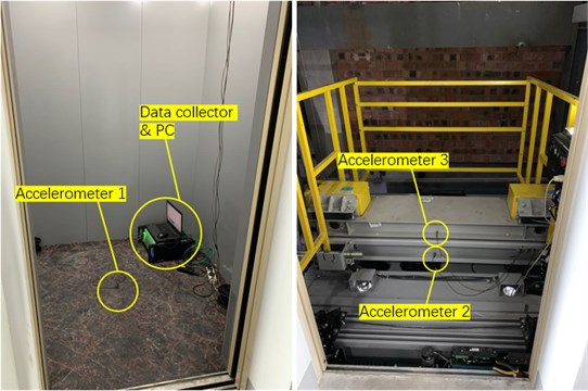
Fig. 5Free vibration signals gathered from three accelerometers when car is near 6th floor, 100 % load condition

3) Repeat measurement under 100 % load condition.

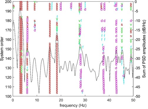
4) Recognize the NFs and damping ratios (DRs) by applying eigensystem realization algorithm (ERA) [15] with natural excitation technique (NExT) [16], stabilization diagrams are used to pick frequencies. An example of stabilization diagram is shown as Fig. 6.

5) Compare experimental results with numerical results.

There are some explanations and details should be noticed:

1) Elevator is a time-variant system during its operation, natural characteristics also change with time. To show this change, free vibration responses are measured then NFs and DRs are identified on discrete measurement positions.

2) Since it is hard to generate enough exciting force that drive the MDOF system to vibrate at a low frequency by a hammer, mechanical braking is performed to excite the system via inertia.

3) Limited by the large operating height, only three measurement points on car side are selected to place accelerometers for the convenience of measurement. In this experiment, mode shapes of the entire system are not focused, 3 points are enough to capture NFs of interest.

4) Subsequent analysis is completed by ERA programmed in MATLAB. Follow the NExT scheme, the correlations between three measured outputs are used as an alternative of the correlations between input and outputs. Specially, three outputs are also regarded as multi-reference channels to improve the performance of the algorithm. Accordingly, Hankel matrix used in ERA has size of $a p \times b q$ , where $p$ and $q$ are number of input and output which are all 3 here, $a$ and $b$ are optional parameters which are chosen from a range of 400 to 500 for the balance of recognizing effect and computational cost.

5) For the clearance of stabilization diagrams, the filtering criteria are chosen as: 1 % for stable NF, 10% for stable DR, consistent mode indicator (CMI) [17] is applied and a relatively loose threshold for CMI is selected as 50 % because the measurement points are few. Sums of power spectral density (PSD) amplitudes are plotted as assistance at the same time.

Fig. 6Stabilization diagram when car is near 6th floor, 100 % load condition: “s” – a pole is stable at NF, DR and CMI at the same time; “d” – stable at both NF and DR; “v” – stable at both NF and CMI; “f” – stable at NF only, dB/Hz – 10 log10 (Amplitude)

Stabilization diagram when car is near 6th floor, 100 % load condition: “s” – a pole is stable at NF, DR and CMI at the same time; “d” – stable at both NF and DR; “v” – stable at both NF and CMI; “f” – stable at NF only, dB/Hz – 10 log10 (Amplitude)

5. Results

The recognized NFs and DRs are listed in Table 2 and Table 3. Due to the complexity of the real elevator installation, measured responses may contain modes that current model cannot reflect, corresponding parameters are listed as column “unknown”. Frequency values with negative damping ratio are discarded. Only the first five orders are presented because the large variation range of natural frequency above the sixth order makes it difficult to extract reliable values.

Table 2Recognized parameters under 0 % load condition

NF (Hz)
Floor	Order
Floor	1st	2nd	Unknown	Unknown	3rd	4th	5th
2F	3.45	4.87	6.90	10.22	14.26	18.10	18.98
3F	3.44	4.23	6.91	10.18	\	17.09	\
4F	3.39	3.85	6.44	10.74	\	\	20.13
5F	3.37	3.64	6.55	\	13.41	17.60	19.66
6F	3.40	4.05	6.68	8.31	10.25	13.44	18.57
7F	3.09	4.43	6.31	8.99	\	\	\
8F	\	4.70	7.09	8.30	9.60	13.92	20.16
DR (%)
2F	7.12	5.43	3.87	0.40	2.55	1.53	0.82
3F	7.34	18.52	6.87	0.38	\	1.12	\
4F	8.14	4.18	10.41	4.41	\	\	1.49
5F	17.01	6.80	8.70	\	4.38	0.80	0.97
6F	13.30	4.67	7.59	8.94	1.74	4.38	0.92
7F	7.80	10.02	7.62	2.52	\	\	\
8F	\	9.64	4.60	2.71	0.96	1.61	3.81

Table 3Recognized parameters under 100 % load condition

NF (Hz)
Floor	Order
Floor	1st	2nd	Unknown	Unknown	3rd	4th	5th
2F	2.65	4.46	\	\	14.54	15.93	20.37
3F	2.76	4.16	\	\	\	16.24	23.34
4F	2.86	4.09	6.07	\	\	14.58	19.06
5F	2.96	3.42	6.21	9.01	\	15.61	17.88
6F	3.07	3.65	6.07	9.05	\	15.32	18.32
7F	2.90	3.86	\	\	11.62	15.75	18.66
8F	2.96	3.39	6.12	\	\	\	17.88
DR (%)
2F	7.97	5.64	\	\	2.66	1.78	2.77
3F	7.30	2.86	\	\	\	1.22	0.51
4F	5.99	1.68	8.21	\	\	1.95	0.90
5F	6.49	6.82	6.18	0.72	\	3.08	2.43
6F	6.31	3.32	7.69	3.00	\	2.30	0.60
7F	6.13	6.56	\	\	2.20	1.39	0.90
8F	7.12	10.67	5.31	\	\	\	0.20

Although the unknown modal parameters are not discussed here, they are still noteworthy in engineering practice since these NF values have the possibility to cause resonance. The appearance of these parameters also indicates that a practical test is important to master the comprehensive status of a real elevator installation.

Fig. 7 shows the comparison of NFs between numerical results and experimental results under 0 % load condition, and Fig. 8 shows the comparison under 100 % load condition. Because DRs are small, damped NFs obtained from the test are used for a roughly comparison to the undamped numerical values. Relative errors between numerical and experimental values for both conditions are listed in Table. 4 and Table. 5.

Fig. 7Comparison of NFs between numerical results and experimental results under 0 % load condition

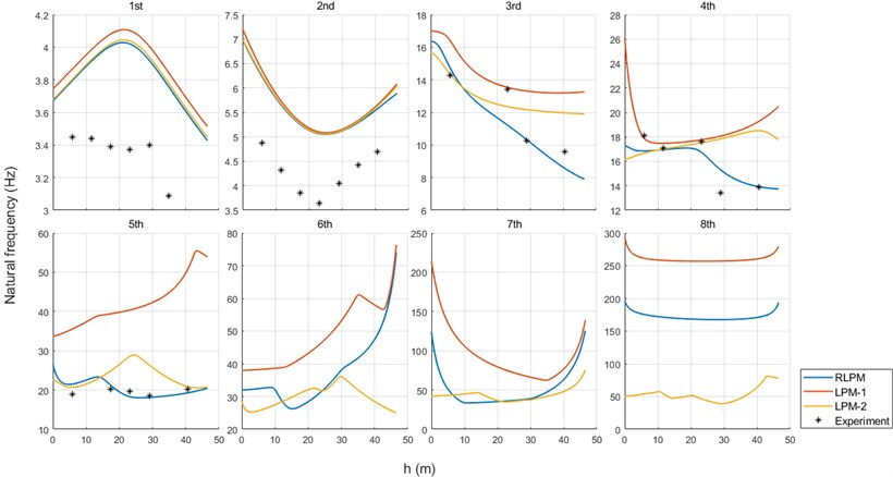
It can be seen from Fig. 7 and Fig. 8, under both conditions, frequency values computed by three models are basically consistent for the first two orders, but differences can be seen since the 3rd order. Curves of RLPM show a faster decrease when $h$ is higher than 20 m for the 3rd the 4th orders and show a flatter change for the 5th order. For the 6th, the 7th and the 8th orders, curves of RLPM present like a compromise of curves of LPM-1 and LPM-2.

Fig. 8Comparison of NFs between numerical results and experimental results under 100 % load condition

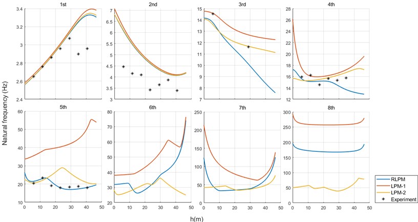
Table 4Relative errors between experimental values and the numerical values under 0 % load condition: R-RLPM; 1-LPM-1; 2-LPM-2

Relative error (%)
Order	1st			2nd			3rd			4th			5th
Floor	Model			Model			Model			Model			Model
Floor	R	1	2	R	1	2	R	1	2	R	1	2	R	1	2
2F	10.11	12.17	10.34	28.22	30.88	28.74	3.52	15.23	0.74	6.94	1.10	7.94	13.21	87.08	9.13
3F	13.74	15.78	14.01	33.64	35.56	34.15	\	\	\	0.80	2.22	0.53	\	\	\
4F	18.30	20.49	18.68	36.21	37.62	36.59	\	\	\	\	\	\	5.38	95.79	23.54
5F	19.26	21.70	19.80	38.90	39.90	39.13	16.29	0.97	7.82	4.89	0.89	0.45	7.05	105.41	45.36
6F	15.21	17.74	15.83	25.89	26.67	26.11	0.77	29.84	18.73	13.88	34.46	32.77	2.52	125.76	41.89
7F	21.84	24.62	22.52	19.33	20.30	19.79	\	\	\	\	\	\	\	\	\
8F	\	\	\	18.62	20.34	19.75	10.83	37.45	24.66	0.00	38.51	33.00	4.40	151.88	3.49

Table 5Relative errors between experimental values and the numerical values under 100 % load condition: R-RLPM; 1-LPM-1; 2-LPM-2

Relative error (%)
Order	1st			2nd			3rd			4th			5th
Floor	Model			Model			Model			Model			Model
Floor	R	1	2	R	1	2	R	1	2	R	1	2	R	1	2
2F	0.01	0.74	0.09	36.29	39.70	36.77	5.33	0.26	6.58	2.02	10.01	3.81	5.40	74.28	1.28
3F	0.00	0.68	0.10	31.35	33.87	31.89	\	\	\	6.78	0.95	5.79	1.52	63.16	5.52
4F	0.44	1.09	0.55	21.85	23.88	22.33	\	\	\	4.18	9.53	6.30	11.25	106.72	30.47
5F	1.03	1.69	1.17	34.68	36.77	35.17	\	\	\	3.01	3.60	1.18	0.38	125.79	59.83
6F	1.68	2.44	1.88	18.32	20.04	18.69	\	\	\	5.44	8.17	5.71	7.28	128.82	43.83
7F	11.98	13.17	12.34	7.00	8.35	7.27	20.83	7.51	1.16	13.07	9.12	6.12	7.23	139.48	23.18
8F	12.18	14.06	12.73	20.05	21.06	20.27	\	\	\	\	\	\	1.48	183.89	15.91

Systematic deviations between numerical and experimental values cause large relative error especially for the 1st and the 2nd orders under 0 % load condition and the 2nd order under 100 % load condition, which might be attributed to the simplification of the model and the estimation of parameters. Numerical results are acceptable considering the inaccuracy in engineering application. For the 3rd and the 4th orders, experimental points under 0 % load condition match the numerical curves of RLPM well, but for 100 % load condition, the advantages of the RLPM have not been proven. However, for the 5th order, it is obvious that experimental points fit the curves of RLPM best under both conditions, relative error analysis shows that RLPM has a certain improvement.

6. Conclusions

In this work, a vertical vibration model for 2:1-ropping elevator system is established, then modal test procedure using ERA is designed to verify the model on calculation of NFs. Conventional LPMs without and with the masses of ropes for the same configuration are also used to compare to the proposed model. The effectiveness of proposed model is validated by comparison results, improvement can be observed in computing the 5th order NFs more accurate under both 0 % load condition and 100 % load condition.

The model proposed in this paper is a development of LPM, which has been proved to have advantages for engineering and research use. The modeling method is also suitable for configurations with larger roping ratio. The mentioned test routine may inspire general engineering practices.

References

X. Arrasate et al., “The modelling, simulation and experimental testing of the dynamic responses of an elevator system,” Mechanical Systems and Signal Processing, Vol. 42, pp. 258–282, 2014.

Publisher
Yue-Qi Zhou, “Models for an elevator hoistway vertical dynamic system,” in 5th International Congress on Sound and Vibration, 1997.

Search CrossRef
S. Watanabe, T. Okawa, D. Nakazawa, and D. Fukui, “Vertical vibration analysis for elevator compensating sheave,” Journal of Physics: Conference Series, Vol. 448, No. 1, p. 012007, Jul. 2013, https://doi.org/10.1088/1742-6596/448/1/012007

Publisher
Jun-Koo Kang and Seung-Ki Sul, “Vertical-vibration control of elevator using estimated car acceleration feedback compensation,” IEEE Transactions on Industrial Electronics, Vol. 47, No. 1, pp. 91–99, 2000, https://doi.org/10.1109/41.824130

Publisher
E. Esteban, O. Salgado, A. Iturrospe, and I. Isasa, “Model-based approach for elevator performance estimation,” Mechanical Systems and Signal Processing, Vol. 68-69, pp. 125–137, Feb. 2016, https://doi.org/10.1016/j.ymssp.2015.07.005

Publisher
B. Z. Knezevic, B. Blanusa, and D. P. Marcetic, “A synergistic method for vibration suppression of an elevator mechatronic system,” Journal of Sound and Vibration, Vol. 406, pp. 29–50, Oct. 2017, https://doi.org/10.1016/j.jsv.2017.06.006

Publisher
D. Mei, X. Du, and Z. Chen, “Optimization of dynamic parameters for a traction-type passenger elevator using a dynamic byte coding genetic algorithm,” Proceedings of the Institution of Mechanical Engineers, Part C: Journal of Mechanical Engineering Science, Vol. 223, No. 3, pp. 595–605, Mar. 2009, https://doi.org/10.1243/09544062jmes1149

Publisher
R. Roberts, “Control of high-rise/high-speed elevators,” in American Control Conference, 1998.

Publisher
Xabier Arrasate, Stefan Kaczmarczyk, Gaizka Almandoz, José M. Abete, and Inge Isasa, “The modeling and experimental testing of the vertical dynamic response of an elevator system with a 2:1 roping configuration.,” in 25th International Conference on Noise and Vibration engineering (ISMA2012), Sep. 2012.

Search CrossRef
S. Kaczmarczyk, “The passage through resonance in a catenary-vertical cable hoisting system with slowly varying length,” Journal of Sound and Vibration, Vol. 208, No. 2, pp. 243–269, Nov. 1997, https://doi.org/10.1006/jsvi.1997.1220

Publisher
S. Kaczmarczyk and W. Ostachowicz, “Transient vibration phenomena in deep mine hoisting cables. Part 1: Mathematical model,” Journal of Sound and Vibration, Vol. 262, No. 2, pp. 219–244, Apr. 2003, https://doi.org/10.1016/s0022-460x(02)01137-9

Publisher
D.-H. Yang, K.-Y. Kim, M. K. Kwak, and S. Lee, “Dynamic modeling and experiments on the coupled vibrations of building and elevator ropes,” Journal of Sound and Vibration, Vol. 390, pp. 164–191, Mar. 2017, https://doi.org/10.1016/j.jsv.2016.10.045

Publisher
R. S. Crespo, S. Kaczmarczyk, P. Picton, and H. Su, “Modelling and simulation of a stationary high-rise elevator system to predict the dynamic interactions between its components,” International Journal of Mechanical Sciences, Vol. 137, pp. 24–45, Mar. 2018, https://doi.org/10.1016/j.ijmecsci.2018.01.011

Publisher
Y. Zhang, S. K. Agrawal, and P. Hagedorn, “Longitudinal vibration modeling and control of a flexible transporter system with arbitrarily varying cable lengths,” Journal of Vibration and Control, Vol. 11, No. 3, pp. 431–456, Mar. 2005, https://doi.org/10.1177/1077546305047988

Publisher
J.-N. Juang and R. S. Pappa, “An eigensystem realization algorithm for modal parameter identification and model reduction,” Journal of Guidance, Control, and Dynamics, Vol. 8, No. 5, pp. 620–627, Sep. 1985, https://doi.org/10.2514/3.20031

Publisher
J. M. Caicedo, “Practical guidelines for the natural excitation technique (NExT) and the eigensystem realization algorithm (ERA) for modal identification using ambient vibration,” Experimental Techniques, Vol. 35, No. 4, pp. 52–58, Jul. 2011, https://doi.org/10.1111/j.1747-1567.2010.00643.x

Publisher
R. S. Pappa, K. B. Elliott, and A. Schenk, “Consistent-mode indicator for the eigensystem realization algorithm,” Journal of Guidance, Control, and Dynamics, Vol. 16, No. 5, pp. 852–858, Sep. 1993, https://doi.org/10.2514/3.21092

Publisher

About this article

Received

11 October 2021

Accepted

18 November 2021

Published

17 March 2022

SUBJECTS

Mechanical vibrations and applications

DOI

https://doi.org/10.21595/jve.2021.22243

Keywords

traction elevator

vertical vibration model

natural frequency

eigensystem realization algorithm

Acknowledgements

This study is sponsored by Zhejiang Province Key Research and Development projects, No. 2020C01084.

The authors would like to give special thanks to Zhejiang Xizi Heavy Industry Machinery Co. Ltd., Jiaxing, China, who has provided essential site and instruments for experiment.

This is an open access article distributed under the Creative Commons Attribution License, which permits unrestricted use, distribution, and reproduction in any medium, provided the original work is properly cited.

Previous article in issue Previous Next article in issue Next

Research article

2024 01 21

Research on estimation and control methods of natural frequency of irregular building structure vibration

Guicai Song

Research article

2020 05 07

Experimental modal analysis and optimal design of cab’s isolation system for a single drum vibratory roller

Le Van Quynh, Zhang Jianrun, Nguyen Van Liem, Bui Van Cuong, Le Xuan Long, Do Thanh Phuong

Research article

2020 02 15

Effect of vehicle-track vertical coupling vibrations on frame-mounted traction motor dynamics

Yuewei Yu, Leilei Zhao, Changcheng Zhou

Research article

2017 05 15

Numerical computation for vibration characteristics of long-span bridges with considering vehicle-wind coupling excitations based on finite element and neural network models

Ling-bo Wang, Pei-wen Jiang

J. Shi, W. Zhang, and C. Wu, “Vertical vibration modeling for 2:1-roping traction elevator system,” Journal of Vibroengineering, Vol. 24, No. 2, pp. 290–304, Mar. 2022, https://doi.org/10.21595/jve.2021.22243

Copy Extrica

Copied to clipboard!

TY  - JOUR
DO  - 10.21595/jve.2021.22243
UR  - https://doi.org/10.21595/jve.2021.22243
TI  - Vertical vibration modeling for 2:1-roping traction elevator system
T2  - Journal of Vibroengineering
AU  - Shi, Jipeng
AU  - Zhang, Weimin
AU  - Wu, Chengjun
PY  - 2022
DA  - 2022/03/17
PB  - JVE International Ltd.
SP  - 290-304
IS  - 2
VL  - 24
SN  - 1392-8716
SN  - 2538-8460
ER  - 

Copy Ris

Copied to clipboard!

@article{Shi_2022,
	doi = {10.21595/jve.2021.22243},
	url = {https://doi.org/10.21595/jve.2021.22243},
	year = 2022,
	month = {mar},
	publisher = {{JVE} International Ltd.},
	volume = {24},
	number = {2},
	pages = {290--304},
	author = {Jipeng Shi and Weimin Zhang and Chengjun Wu},
	title = {Vertical vibration modeling for 2:1-roping traction elevator system},
	journal = {Journal of Vibroengineering}
}

Copy Bibtex

Copied to clipboard!

[1]J. Shi, W. Zhang, and C. Wu, “Vertical vibration modeling for 2:1-roping traction elevator system,” Journal of Vibroengineering, vol. 24, no. 2, pp. 290–304, Mar. 2022, doi: 10.21595/jve.2021.22243.

Copy IEEE

Copied to clipboard!

Shi, Jipeng, Weimin Zhang, and Chengjun Wu. “Vertical Vibration Modeling for 2:1-Roping Traction Elevator System.” Journal of Vibroengineering 24, no. 2 (March 17, 2022): 290–304. https://doi.org/10.21595/jve.2021.22243.

Copy Chicago

Copied to clipboard!

Vertical vibration modeling for 2:1-roping traction elevator system

Abstract

Highlights

1. Introduction

2. Vertical vibration model

2.1. Model description

2.2. Equations of motion

3. Numerical and experimental verification

4. Experimental procedure

5. Results

6. Conclusions

References

About this article

Related Articles