Dynamics of a three-mass system with cubic nonlinearity and that of an equivalent electrical circuit

Nikishins, Vladimirs; Grinevichs, Ivans; Scukins, Igors

doi:10.21595/jve.2022.22539

Journal of Vibroengineering

Browse Journal

Submit article

Published: 11 November 2022

Check for updates

Dynamics of a three-mass system with cubic nonlinearity and that of an equivalent electrical circuit

Vladimirs Nikishins¹

Ivans Grinevichs²

Igors Scukins³

^{1, 2, 3}RTU Daugavpils Study and Science Centre, Riga Technical University, Daugavpils, Latvia

Corresponding Author:

Vladimirs Nikishins

Cite the article Download PDF

Downloads 303

Abstract

The paper considers the reaction of a mechanical system of three masses connected by springs and absorbers moving in the longitudinal direction to the action of a harmonic force applied to the largest mass. This mass is attached to the base by a spring with cubic nonlinearity, while smaller masses are connected to the main mass by linear springs. A method is proposed for obtaining the amplitude-frequency characteristic (AFC) of a nonlinear system from the AFC sequence of linearized systems. The results of modelling an equivalent electrical circuit, which is an analogue of a mechanical system, are presented. The influence of the value of the nonlinearity coefficient on the dynamic response of systems has been studied. It is noted that for some combinations of values of the system parameters with cubic nonlinearity with mass ratios $m_{1}$ : $m_{2}$ : $m_{3}$ = 4:2:1, the AFC contains outer and inner isolated areas – islands.

1. Introduction

Models of two or three masses connected by nonlinear springs and absorbers are often used to describe various mechanisms: vibration isolation systems such as a suspension of a vehicle, an industrial robot cutting arm, a punching press, an impact tool, a gyroscope, a generator. The vehicle suspension is modelled in [1-5] by a system of three masses with springs and absorbers. The system parameters that ensure the driver’s comfort and safety are determined using a wavelet analysis. In [6-9] a system with two degrees of freedom consists of a large-mass linear oscillator and a low-mass nonlinear vibration absorber. Free and forced oscillations of the system are studied using the theory of normal modes and perturbation methods. In [7], the dynamics of a linear oscillator is studied for a similar model by the averaging method. The goal is to reduce the amplitude of the oscillator near resonance by adjusting the parameters of the nonlinear absorber. It is shown that both a positive influence of a nonlinear absorber and a negative one in the appearance of unstable modes leading to dangerous instability, are possible. Various complex motions associated with these instabilities are studied by the method of direct numerical integration.

The universal software package SPRING, designed to study various problems of the dynamics of nonlinear systems, was used in to study the bifurcations of single-mass systems with different types of nonlinearities.

The vibration microgyroscope in [10] consists of three masses, two masses oscillate in the longitudinal direction, and the third one can also oscillate in the transverse direction, absorbing the vibrations of the active mass. This design, in combination with the proposed technological methods, improves the quality of the gyroscope. In [11], a model of a vibro-impact triboelectric generator with three degrees of freedom is presented. The impact of various ratios of masses and distances between them on the dynamic response and the generated energy has been studied. It is concluded that symmetric mass configurations of the oscillator are energetically more favourable than asymmetric cases.

The aim of paper [12] is to analyse the discrete dynamic behaviour of nonlinear intelligent mechanical vibration systems with co-located sensors and actuating units. To illustrate the theory, a numerical example of a system with two masses is given. The considered approach is proposed to be applied to systems with three masses.

2. Equations of motion

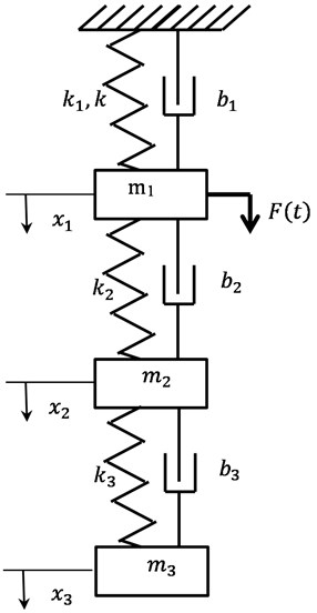
The mechanical system (MS) is described (Fig. 1) by the system of equations:

1

\{\begin{array}{l} m_{1} {\ddot{x}}_{1} + (b_{1} + b_{2}) {\dot{x}}_{1} - b_{2} {\dot{x}}_{2} + (k_{1} + k_{2}) x_{1} + k x_{1}^{3} - k_{2} x_{2} = F_{m} \sin (ω t), \\ m_{2} {\ddot{x}}_{2} - b_{2} {\dot{x}}_{1} + (b_{2} + b_{3}) {\dot{x}}_{2} - b_{3} {\dot{x}}_{3} - k_{2} x_{1} + (k_{2} + k_{3}) x_{2} - k_{3} x_{3} = 0, \\ m_{3} {\ddot{x}}_{3} - b_{3} {\dot{x}}_{2} + b_{3} {\dot{x}}_{3} - k_{3} x_{2} + k_{3} x_{3} = 0, \end{array}

where $m_{1}$ , $m_{2}$ , $m_{3}$ – masses of bodies; $b_{1}$ , $b_{2}$ , $b_{3}$ – damping coefficient; $k_{1}$ , $k_{2}$ , $k_{3}$ – linear coefficients of spring stiffness; $k$ – nonlinear coefficient of the 1st spring ( $k_{1} x + k x^{3}$ – cubic nonlinearity); $F_{m}$ – amplitude of the harmonic force applied to the 1st mass.

Fig. 1Mechanical system with three masses

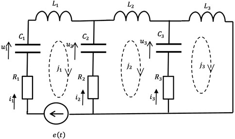
The electrical circuit (EC) is described (Fig. 2) by a system of equations compiled according to the method of loop currents:

2

\{\begin{array}{l} L_{1} \frac{d j_{1}}{d t} + R_{1} j_{1} + \frac{1}{C_{1}} \int j_{1} d t + R_{2} (j_{1} - j_{2}) + \frac{1}{C_{2}} \int (j_{1} - j_{2}) d t = e (t), \\ L_{2} \frac{d j_{2}}{d t} - R_{2} (j_{1} - j_{2}) - \frac{1}{C_{2}} \int (j_{1} - j_{2}) d t + R_{3} (j_{2} - j_{3}) + \frac{1}{C_{3}} \int (j_{2} - j_{3}) d t = 0, \\ L_{3} \frac{d j_{3}}{d t} + R_{3} (j_{3} - j_{2}) + \frac{1}{C_{3}} \int (j_{3} - j_{2}) d t = 0, \end{array}

where $L_{k}$ – inductance ( $k =$ 1, 2, 3); $R_{k}$ – resistors resistance; $C_{k}$ – capacitor capacity; $j_{k}$ – loop currents. Given that the amount of electricity from the loop current $Q_{k} = \int j_{k} d t$ , the system of equations of the loop current method (2) can be written in the following form:

3

\{\begin{array}{l} L_{1} {\ddot{Q}}_{1} + (R_{1} + R_{2}) {\dot{Q}}_{1} - R_{2} {\dot{Q}}_{2} + (S_{1} + S_{2}) Q_{1} + S Q_{1}^{3} - S_{2} Q_{2} = E_{m} \sin (ω t), \\ L_{2} {\ddot{Q}}_{2} - R_{2} {\dot{Q}}_{1} + (R_{2} + R_{3}) {\dot{Q}}_{2} - R_{3} {\dot{Q}}_{3} - S_{2} Q_{1} + (S_{2} + S_{3}) Q_{2} - S_{3} Q_{3} = 0, \\ L_{3} {\ddot{Q}}_{3} - R_{3} {\dot{Q}}_{2} + R_{3} {\dot{Q}}_{3} - S_{3} Q_{2} + S_{3} Q_{3} = 0, \end{array}

where $S_{k} = 1 / C_{k}$ – inverse capacitance, $S =$ 0 for the linear system, $E_{m}$ – amplitude of harmonic voltage of the generator.

Fig. 2Equivalent electrical circuit

Capacitor currents are expressed in terms of loop currents:

4

\{\begin{array}{l} i_{1} = j_{1}, \\ i_{2} = j_{2} - j_{1}, \\ i_{3} = j_{3} - j_{2}, \end{array}

and the charges (amounts of electricity) of the capacitors are equal to $q_{k} = \int i_{k} d t$ , then the ratios for the quantities of electricity of capacitors and the quantities of electricity from loop currents are true:

5

\{\begin{array}{l} q_{1} = Q_{1}, \\ q_{2} = Q_{2} - Q_{1}, \\ q_{3} = Q_{3} - Q_{2}, \end{array}

and the voltages of the capacitors are found by the formulas $u_{1} = S_{1} q_{1} + S {(q_{1})}^{3}$ , $u_{k} = S_{k} q_{k}$ ( $k =$ 2, 3). To reduce the equations of motion of a mechanical system to dimensionless parameters, the following expressions are used:

m_{0} = m_{3}, x_{0} = \frac{F_{m}}{k_{3}}, t_{0} = 2 π \sqrt{\frac{m_{0}}{k_{3}}}, {\tilde{m}}_{k} = \frac{m_{k}}{m_{0}}, {\tilde{x}}_{k} = \frac{x_{k}}{x_{0}}, \tilde{t} = \frac{t}{t_{0}}, \tilde{ω} = ω t_{0},

{\tilde{b}}_{k} = b_{k} \frac{t_{0}}{m_{0}}, {\tilde{k}}_{k} = k_{k} \frac{t_{0}^{2}}{m_{0}}, \tilde{k} = k \frac{x_{0}^{2} ∙ t_{0}^{2}}{m_{0}}, {\tilde{F}}_{m} = F_{m} \frac{t_{0}^{2}}{m_{0} x_{0}}, (k = 1,2, 3),

where the sign “~” denotes dimensionless parameters. After substituting these expressions and transformations into the system of differential equations of motion of a mechanical system, a system of equations in dimensionless parameters will be obtained. The form of the resulting system of equations, after discarding the “~” sign from the symbols, coincides with the form of the dimensional system. The above equations of motion of a mechanical system are also true for dimensionless parameters.

To reduce the equations of motion of the electrical system to dimensionless parameters, the following expressions are used:

L_{0} = L_{3}, Q_{0} = \frac{E_{m}}{S_{3}}, t_{0} = 2 π \sqrt{\frac{L_{0}}{S_{3}}}, {\tilde{L}}_{k} = \frac{L_{k}}{L_{0}}, {\tilde{Q}}_{k} = \frac{Q_{k}}{Q_{0}}, \tilde{t} = \frac{t}{t_{0}}, \tilde{ω} = ω t_{0},

{\tilde{R}}_{k} = R_{k} \frac{t_{0}}{L_{0}}, {\tilde{S}}_{k} = S_{k} \frac{t_{0}^{2}}{L_{0}}, \tilde{S} = S \frac{Q_{0}^{2} ∙ t_{0}^{2}}{L_{0}}, {\tilde{E}}_{m} = E_{m} \frac{t_{0}^{2}}{L_{0} Q_{0}},

{\tilde{u}}_{k} = \frac{u_{k} t_{0}^{2}}{L_{0} Q_{0}}, (k = 1,2, 3),

where the sign “~” denotes dimensionless parameters. Performing operations similarly to the case of a mechanical system leads to a dimensionless system of differential equations of an electrical circuit. The form of the resulting system of equations, after discarding the sign “~” from the symbols, coincides with the form of the dimensional system. The above equations of the electrical system are also true for dimensionless parameters.

Comparison of the equations for MS and EC leads to a well-known analogy between them (Table 1).

Table 1Analogy between the parameters of mechanical and electrical systems

Mass $m_{k}$ , kg	Inductance $L_{k}$ , H
Damping coefficient $b_{k}$ , N·s/m	Resistance $R_{k}$ , Ω
Elastic coefficient $k_{k}$ , N/m	Inverse capacitance $S_{k}$ , F^-1
Mass displacement $x_{k}$ , m	The amount of electricity of the loop current $Q_{k}$ , C
Velocity ${\dot{x}}_{k}$ , m/s	Loop current $j_{k}$ , A
Force of spring elasticity, N	Capacitor voltage $u_{k}$ , V
Force $F_{k}$ , N	Electromotive force $E_{m}$ , V

Taking into account this analogy, the method is described below only for a mechanical system.

Normal form of equations for the mechanical system (Fig. 1):

6

\{\begin{array}{l} {\dot{x}}_{1} = x_{4}, \\ {\dot{x}}_{2} = x_{5}, \\ {\dot{x}}_{3} = x_{6}, \\ {\dot{x}}_{4} = \frac{1}{m_{1}} [F_{m} \sin ω t + k_{2} x_{2} - (k_{1} + k_{2}) x_{1} - k x_{1}^{3} + b_{2} x_{5} - (b_{1} + b_{2}) x_{4}], \\ {\dot{x}}_{5} = \frac{1}{m_{2}} [k_{3} x_{3} - (k_{2} + k_{3}) x_{2} + k_{2} x_{1} + b_{3} x_{6} - (b_{2} + b_{3}) x_{5} + b_{2} x_{4}], \\ {\dot{x}}_{6} = \frac{1}{m_{3}} [k_{3} x_{2} - k_{3} x_{3} - b_{3} x_{6} + b_{3} x_{5}], \end{array}

where $x_{1,2, 3}$ – displacements of the 1st, 2nd, 3rd masses; $x_{4,5, 6}$ – velocity of the 1st, 2nd, 3rd masses; circular frequency 1 $< ω <$ 13; time 0 $< t <$ 70. Parameter values: $m_{1} =$ 4; $m_{2} =$ 2; $m_{3} =$ 1 – masses of bodies; $b_{1} =$ 1; $b_{2} =$ 0.3; $b_{3} =$ 0.3 – damping coefficients; $k_{1} =$ 100; $k_{2} =$ 25; $k_{3} =$ 40 – linear coefficients of spring forces; $k =$ 20…400 nonlinear coefficient of the 1st spring ( $k_{1} x + k x^{3}$ – cubic nonlinearity); $F_{m} =$ 40 – the amplitude of the force applied to the 1st mass. The numerical solution (NS) for a normal system was obtained by the Runge-Kutta method in the SPRING program [13], developed to study dynamic processes in nonlinear systems.

3. Analytical solution method

“Energy” linearization (EL) is the replacement of nonlinear equations with linear ones based on the equality of potential energies of equally deformed nonlinear and equivalent linear springs. Let the force and deformation of a nonlinear spring be related by the relation:

7

F_{n} = k_{1} x + k x^{3},

and for an equivalent linear spring, this relationship has the form:

8

F_{e} = k_{e} x,

where $k_{е}$ – $c o n s t$ , for a specific deformation $х$ . From the equality of potential energies of equally deformed springs:

9

\int_{0}^{x} F_{e} d x = \int_{0}^{x} F_{n} d x, \int_{0}^{x} k_{e} x d x = \int_{0}^{x} k_{1} x + k x^{3} d x,

the equivalent coefficient of elasticity of a linear spring is found:

10

k_{e} (x) = k_{1} + \frac{1}{2} k x^{2} .

With “force” linearization (FL), the forces of equally deformed nonlinear and equivalent linear springs are equated:

11

F_{n} = F_{e},

and the equivalent coefficient of elasticity of the linear spring is found:

12

k_{e} (x) = k_{1} + k x^{2} .

In the general case, the equivalent coefficient of elasticity of a linear spring for a cubic nonlinearity can be written as:

13

k_{e} (x) = k_{1} + s k x^{2},

where $s$ – weight coefficient, 0.5 $\leq s \leq$ 1. The minimum value of the weight coefficient $s =$ 0.5 corresponds to EL, and the maximum value $s =$ 1 corresponds to FL.

Formally, when solving the system of MS equations, we can put $k =$ 0 and $k_{1} = k_{e} (x_{1})$ . The resulting linear system is solved by the method of complex amplitudes, as a result of which the system of differential equations is reduced to a system of linear algebraic equations for complex amplitudes:

14

A ∙ (\begin{matrix} {\dot{X}}_{1} \\ {\dot{X}}_{2} \\ {\dot{X}}_{3} \end{matrix}) = (\begin{matrix} F_{m} \\ 0 \\ 0 \end{matrix}),

where ${\dot{X}}_{n} = X_{n} ∙ e^{j ∙ φ_{n}}$ – complex displacement amplitude $x_{n}$ ( $n =$ 1, 2, 3); hereinafter, the dot above the symbol denotes the complex nature of the value , and not differentiation with respect to time, as it was in the systems of equations, $j = \sqrt{- 1}$ – imaginary unit; $x_{n} = I m ({\dot{X}}_{n} e^{j ∙ ω t}) = X_{n} \sin (ω t + φ_{n})$ ; $A$ – matrix of coefficients with elements $a_{11} = - m_{1} ω^{2} + j ω (b_{1} + b_{2}) + k_{e} + k_{2}$ , $a_{12} = - k_{2} - j ω b_{2}$ , $a_{13} = 0$ , $a_{21} = - k_{2} - j ω b_{2}$ , $a_{22} = - m_{2} ω^{2} + j ω (b_{2} + b_{3}) + k_{2} + k_{3}$ , $a_{23} = - k_{3} - j ω b_{3}$ , $a_{31} = 0$ , $a_{32} = - k_{3} - j ω b_{3}$ , $a_{33} = k_{3} + j ω b_{3} - m_{3} ω^{2}$ .

According to Cramer’s formulae, the solution to the system of linear algebraic equations of complex amplitudes has the form:

15

{\dot{X}}_{n} = \frac{∆_{n}}{d e t A (ω, k_{e})}, (n = 1,2, 3),

where the numerator and denominator are complex polynomials with respect to frequency $ω$ . For example:

16

∆_{n} = A_{n} (F_{m}, ω) + j B_{n} (F_{m}, ω),

where

A_{1} (F_{m}, ω) = F_{m} (m_{2} m_{3} ω^{4} - (b_{2} b_{3} + k_{2} m_{3} + k_{3} m_{2} + k_{3} m_{3}) ω^{2} + k_{2} k_{3}),

B_{1} (F_{m}, ω) = F_{m} (- (b_{2} m_{3} + b_{3} m_{2} + b_{3} m_{3}) ω^{3} + (b_{2} k_{3} + b_{3} k_{2}) ω),

A_{2} (F_{m}, ω) = F_{m} (- (b_{2} b_{3} + k_{2} m_{3}) ω^{2} + k_{2} k_{3}),

B_{2} (F_{m}, ω) = F_{m} (- (b_{2} m_{3}) ω^{3} + (b_{2} k_{3} + b_{3} k_{2}) ω),

A_{3} (F_{m}, ω) = F_{m} (- (b_{2} b_{3}) ω^{2} + k_{2} k_{3}),

B_{3} (F_{m}, ω) = F_{m} (b_{2} k_{3} + b_{3} k_{2}) ω .

Moduli of complex amplitudes:

17

X_{n} = \frac{{| ∆}_{n} |}{| d e t A (ω, k_{e}) |}, (n = 1,2, 3),

after squaring:

18

X_{n}^{2} = \frac{{{| ∆}_{n} |}^{2}}{{| d e t A ({ω, k}_{e}) |}^{2}},

will be the ratio of real polynomials with respect to frequency $ω$ . Expression for $d e t A (ω, k_{e})$ with Eq. (12) for FL:

19

k_{e} = k_{1} + k ∙ X_{1}^{2},

will be as follows:

20

d e t A (ω, X_{1}) = U (ω) + j W (ω) + Z (ω) X_{1}^{2} + j T (ω) X_{1}^{2},

where:

21

T (ω) = k (ω (b_{2} k_{3} + b_{3} k_{2}) + ω^{3} ((- b_{3} - b_{2}) m_{3} - b_{3} m_{2})),

Z (ω) = k (k_{2} k_{3} - ω^{2} ((k_{3} + k_{2}) m_{3} + (k_{3} m_{2} + b_{2} b_{3})) + ω^{4} m_{2} m_{3}) .

The polynomials $U (ω)$ and $W (ω)$ can be written as the scalar product of vectors:

22

U (ω) = (\begin{matrix} \begin{matrix} U_{1} & U_{2} \end{matrix} & \begin{matrix} U_{3} & U_{4} \end{matrix} \end{matrix}) (\begin{matrix} \begin{matrix} 1 \\ ω^{2} \end{matrix} \\ \begin{matrix} ω^{4} \\ ω^{6} \end{matrix} \end{matrix}),

where the coordinates of the first term are the coefficients of a polynomial with even powers of the cyclic frequency:

23

U_{1} = k_{1} k_{2} k_{3},

U_{2} = (((k_{2} + k_{1}) k_{3} + k_{1} k_{2}) m_{3} + (k_{2} + k_{1}) k_{3} m_{2} + k_{2} k_{3} m_{1} + b_{1} b_{2} k_{3} + b_{1} b_{3} k_{2} + b_{2} b_{3} k_{1}),

U_{3} = ((k_{2} + k_{1}) m_{2} + (k_{3} + k_{2}) m_{1} + (b_{2} + b_{1}) b_{3} + b_{1} b_{2}) m_{3} + (k_{3} m_{1} + (b_{2} + b_{1}) b_{3}) m_{2} + b_{2} b_{3} m_{1},

U_{4} = - m_{1} ∙ m_{2} {∙ m}_{3} .

Similarly:

24

W (ω) = (\begin{matrix} \begin{matrix} W_{1} & W_{2} \end{matrix} & W_{3} \end{matrix}) (\begin{matrix} ω \\ \begin{matrix} ω^{3} \\ ω^{5} \end{matrix} \end{matrix}),

here the coordinates of the first vector are the coefficients of a polynomial with odd powers of cyclic frequency:

25

W_{1} = (b_{1} k_{2} + b_{2} k_{1}) k_{3} + b_{3} k_{1} k_{2},

W_{2} = (((b_{2} + b_{3}) k_{3} + (b_{3} + b_{1}) k_{2} + (b_{3} + b_{2}) k_{1}) m_{3} + ((b_{2} + b_{1}) k_{3} + b_{3} k_{2} + b_{3} k_{1}) m_{2} + (b_{2} k_{3} + b_{3} k_{2}) m_{1} + b_{1} b_{2} b_{3}),

W_{3} = ((b_{2} + b_{1}) m_{2} + (b_{3} + b_{2}) m_{1}) m_{3} + b_{3} m_{1} m_{2} .

Substituting Eq. (20) for $d e t A (ω, X_{1})$ into for Eq. (18) of the squared amplitude for $n =$ 1, after transformations, we obtain the expression:

26

X_{1}^{2} = \frac{A_{1}^{2} (F_{m}, ω) + B_{1}^{2} (F_{m}, ω)}{{(Z (ω) ∙ X_{1}^{2} + U (ω))}^{2} + {(T (ω) ∙ X_{1}^{2} + W (ω))}^{2}},

which is a cubic equation with respect to the square of the modulus ${(X_{1})}^{2}$ :

27

({Z (ω)}^{2} + {T (ω)}^{2}) ∙ X_{1}^{6} + 2 (U (ω) Z (ω) + W (ω) T (ω)) ∙ X_{1}^{4} + ({U (ω)}^{2} + {W (ω)}^{2}) ∙ X_{1}^{2} - {A_{1} (F_{m}, ω)}^{2} - {B_{1} (F_{m}, ω)}^{2} = 0 .

By setting $ω$ , roots $X_{1}$ are found from this equation and the amplitude-frequency characteristic (AFC) is constructed for the first approximation of the nonlinear system. With one real root of the cubic equation, MS has one stable mode, and with three real roots, two stable and one unstable modes. The ambiguity $X_{1}$ is taken into account when determining the displacement amplitudes of other masses $X_{2}$ and $X_{3}$ . The described method was implemented in the Mathcad software.

4. Graphic analogue of the method

The method presented above is an analytical implementation of a graphical method for determining AFC of the nonlinear MS from AFC of the linear MS. Graphically, the AFC of the nonlinear MS can be found from the AFC of the linear MS using the following algorithm:

1. Set the initial value of displacement $x_{1}$ ;

2. Determine the coefficient of equivalent stiffness of the nonlinear MC for the given displacement $k_{e} (x_{1})$ according to the chosen linearization method (EL, FL);

3. Assume the parameter $k_{1}$ of a linear MS to be equal to the coefficient of equivalent stiffness $k_{1} = k_{e} (x_{1})$ ;

4. Construct the AFC of the linear MS of point 3;

5. Draw a horizontal line L at level $x_{1}$ on the AFC of point 4;

6. Determine the coordinates of the points of intersection of line L with the AFC. If there are no intersection points, then exit the algorithm;

7. The points in 6 belong to the AFC of the nonlinear MS and are marked on its graph;

8. The displacement value х₁ is increased by the amount of the selected step. Go to point 2.

If you need to find the AFC of the nonlinear EC, then the graphical method has specific features and is as follows:

1. Set the initial value of the amount of electricity $Q_{1}$ (analogue of displacement $x_{1}$ );

2. Determine the equivalent inverse capacitance $S_{e} (Q_{1}) = S_{1} + S {(Q_{1})}^{2}$ (FL);

3. Parameter $S_{1}$ is assumed to be equal to the equivalent inverse capacitance $S_{1} = S_{e} (Q_{1})$ ;

4. Find capacitance $C_{1} = 1 / S_{1}$ ;

5. Determine dimensional parameter (real capacitance) $C_{r 1}$ ;

6. Determine voltage $u_{1} = S_{1} Q_{1}$ across capacitor $C_{1}$ ;

7. Determine the dimensional parameter (the real voltage across capacitor $C_{r 1}$ ) $u_{r 1} = u_{1} (L_{0} Q_{0}) / t_{0}^{2}$ ;

8. Construct the AFC of the linear EC with capacitor $C_{r 1}$ ;

9. Draw a horizontal line $L$ on the AFC of point 8 at level $u_{r 1}$ ;

10. Determine the coordinates of the points of intersection of line $L$ with the AFC. If there are no intersection points, then exit the algorithm;

11. The points in 10 belong to the AFC of the nonlinear EC and are marked on its graph;

12. The value of the amount of electricity $Q_{1}$ is increased by the value of the selected step. Go to point 2.

An example is given below for the EC graphical algorithm. Let the dimensionless parameters of the MS be known: $m_{1} =$ 4; $m_{2} =$ 2; $m_{3} =$ 1; $b_{1} =$ 1; $b_{2} =$ 0.3; $b_{3} =$ 0.3; $k_{1} =$ 100; $k_{2} =$ 25; $k_{3} =$ 40; $k_{} =$ 60; $F_{m} =$ 40.

Using the analogy between MS and EC, the dimensionless parameters of the EC are found: $L_{1} =$ 4; $L_{2} =$ 2; $L_{3} =$ 1; $R_{1} =$ 1; $R_{2} =$ 0.3; $R_{3} =$ 0.3; $S_{1} =$ 100; $S_{2} =$ 25; $S_{3} =$ 40; $S =$ 60; $E_{m} =$ 40. To obtain the dimensional parameters of EC, three parameters must be set in an arbitrary way, let them be $L_{3} =$ 0.1 H, $C_{3} =$ 470 pF, $E_{m} =$ 1 V, then, using the relationship between the dimensional and dimensionless parameters, the remaining dimensional parameters of the EC are found (4 digits are retained): $L_{1} =$ 0.4 H; $L_{2} =$ 0.2 H; $R_{1} =$ 2322 Ω; $R_{2} =$ 696 Ω; $R_{3} =$ 696 Ω; $C_{1} =$ 185.5 pF; $C_{2} =$ 742.2 pF. The electrical circuit of the dimensional EC is designed in the Multisim program (Fig. 3). The AFC of the linear EC are obtained using the Bode Plotter tool (Fig. 4). By moving the marker along the AFC, the coordinates of the desired points of the curve are determined.

Fig. 3Dimensional EC in the Multisim program

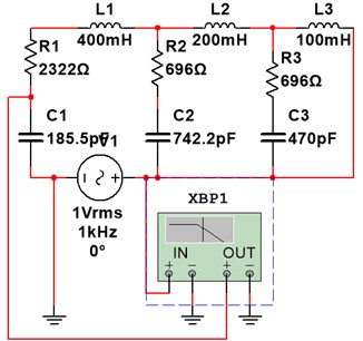
Fig. 4AFC of the dimensional EC in the Bode Plotter tool window of the Multisim program with a movable vertical marker (in the lower part of the window on the left is the frequency and on the right is the corresponding ordinate of the marker’s intersection point with the graph)

AFC of the dimensional EC in the Bode Plotter tool window of the Multisim program with a movable vertical marker (in the lower part of the window on the left is the frequency and on the right is the corresponding ordinate of the marker’s intersection point with the graph)

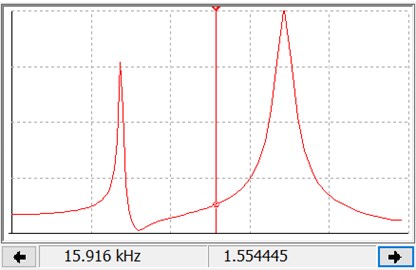
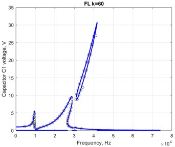
Fig. 5 shows the AFC of the dimensional EC recalculated to the dimensional parameters for FL and the simulation results (graphical algorithm), which the centres of the circles correspond to.

Fig. 5The recalculated AFC of the dimensional EC and the results of the graphical algorithm (centres of circles) obtained in program multisim

5. Results

The results of the influence of a change in the coefficient of nonlinearity к on the shape of the AFC of a three-mass system are presented in the graphs Fig. 6, 7, 8.

Fig. 6AFC of the dimensionless MS at EL for nonlinearity coefficients k= 20, 60 without singularities and at k= 100 with a detached part of the vertex – the “outer island”

AFC of the dimensionless MS at EL for nonlinearity coefficients k= 20, 60 without singularities and at k= 100 with a detached part of the vertex – the “outer island”

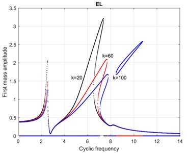
Fig. 7AFC of dimensionless MS at EL for coefficients of nonlinearity k= 140, 260, there is an increase in the size of the “outer island” and at k= 350 the “outer island” joins the vertex with the beginning of the formation of the “inner island” under it

AFC of dimensionless MS at EL for coefficients of nonlinearity k= 140, 260, there is an increase in the size of the “outer island” and at k= 350 the “outer island” joins the vertex with the beginning of the formation of the “inner island” under it

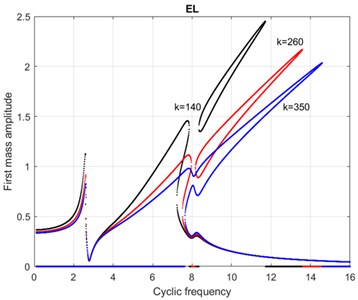
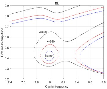
Fig. 8AFC of dimensionless MS at EL for coefficients of nonlinearity k= 450 continuation of the formation of the “inner island”, k= 550 completion of its formation and k= 600 reduction of its size

AFC of dimensionless MS at EL for coefficients of nonlinearity k= 450 continuation of the formation of the “inner island”, k= 550 completion of its formation and k= 600 reduction of its size

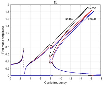
Fig. 9The enlarged part of the graphs in Fig. 8 showing the emergence of an “inner island” and reducing its size (with a further increase in k, the island shrinks to a point and disappears)

The enlarged part of the graphs in Fig. 8 showing the emergence of an “inner island” and reducing its size (with a further increase in k, the island shrinks to a point and disappears)

Graphs for the same nonlinearity coefficients for the EL and FL and their comparison with the NS is demonstrated in Fig. 10, 11.

Fig. 10Comparison of the AFC of the dimensionless MC at EL (there is no “outer island”) and FL (the “outer island” increases and approaches the vertex) with NS (increase in the size of the “outer island” that has arisen) for a coefficient of nonlinearity k= 60 (NS is the numerical integration of the system (6) in SPRING program)

Comparison of the AFC of the dimensionless MC at EL (there is no “outer island”) and FL (the “outer island” increases and approaches the vertex) with NS (increase in the size of the “outer island” that has arisen) for a coefficient of nonlinearity k= 60 (NS is the numerical integration of the system (6) in SPRING program)

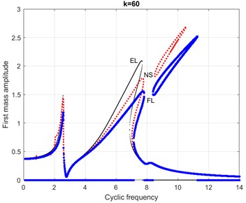
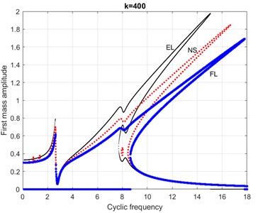
Fig. 11Comparison of the AFC of the dimensionless MS at EL (the beginning of the formation of the “inner island”) and FL (the “inner island” has disappeared) with NS (there is an “inner island”) for a nonlinearity coefficient k= 400

Comparison of the AFC of the dimensionless MS at EL (the beginning of the formation of the “inner island”) and FL (the “inner island” has disappeared) with NS (there is an “inner island”) for a nonlinearity coefficient k= 400

At close to zero values of the nonlinearity coefficient к the AFC of the dimensionless MS has three partial resonances: at $ω_{1} =$ 2.3 and $ω_{2} =$ 6 clearly expressed and at $ω_{3} =$ 8.2 hardly noticeable, what can be seen on the graph Fig. 6. for $k =$ 20 (the slope of the vertex of the second resonance is due to non-linearity). An increase in the nonlinearity coefficient causes a transformation of the AFC, which can be conditionally divided into the following stages:

1) the appearance of an “outer island” of small size (a point). By “outer island” here we mean a separate area of the AFC graph that is not related to the main AFC, having no features. For example, the main AFC in Fig. 6 there will be curves for $k =$ 20 $k =$ 60, and the graph for $k =$ 100 consists of the main curve and the “outer island”. The difference between the “outer island” and the “inner island” is that if you draw a vertical straight line through a separate area of the graph and move along this straight line from the abscissa axis upwards, then for the “outer island” the first point of intersection of the vertical will be with the main AFC, and the second and the third intersection point will be with the boundaries of the “outer island”. For the “inner island”, the first and second points of intersection of the vertical line, when moving up along, will be with the boundaries of the “inner island”, and the third point of intersection will be with the main AFC.

2) Increasing the size of the “outer island”, as seen in Fig. 7 for graphs at $k =$ 140 and $k =$ 260.

3) Contact and merging of the “outer island” with the main AFC, which is illustrated by the graph in Fig. 7 at $k =$ 350.

4) Formation of the “inner island” under the spot of merging (their point 3). This process can be traced in the graphs in Fig. 7 at $k =$ 350 and 8 for $k =$ 450, the merging occurs at the dimensionless cyclic frequency $ω =$ 8.

5) The emergence of the “inner island”, for example, in Fig. 8 at $k =$ 550 and the zoomed image in Fig. 9 at $k =$ 550.

6) The reduction in the size of the “inner island” can be seen in Fig. 8 for $k =$ 600 and zoomed in Fig. 9 for $k =$ 600.

7) The disappearance of the “inner island”, after which the AFC remains, an example of it is given in Fig. 11 for FL.

The curves in Fig.10, 11 show that the MS considered at EL (weight coefficient $s =$ 0.5) is less rigid, and at FL ( $s =$ 1) it is more rigid than the true MS, for which the NS takes place, which is taken here as a benchmark. Any value of the weight coefficient from the interval (0.5;1), for example $s =$ 0.75, will give a smaller deviation of the linearized solution from the benchmark.

6. Conclusions

The paper proposes a method for constructing the AFC of a nonlinear system from the set of the AFC of the corresponding linearized systems. It is shown that the benchmark response of a nonlinear system obtained in the SPRING program is the interval between the responses of systems linearized in force and energy. By choosing the optimal weight coefficient, one can achieve the minimum deviation of the approximate solution from the benchmark. Algorithms for graphical construction of the AFC of a nonlinear mechanical system and an equivalent electrical circuit are presented, which graphically implement the proposed analytical method. The influence of the value of the nonlinearity coefficient on the dynamic response of systems has been studied. It has been shown that for some values of the parameters of systems with cubic nonlinearity, the AFC contains outer and inner isolated areas – islands, and the process of the appearance and disappearance of such islands has been illustrated.

References

K. Nouri, H. Loussifi, and N. B. Braiek, “Modelling and wavelet-based identification of 3-DOF vehicle suspension system,” Journal of Software Engineering and Applications, Vol. 4, No. 12, pp. 672–681, 2011, https://doi.org/10.4236/jsea.2011.412079

Publisher
Zaripov, R., Gavrilovs, and P., “Assessment of the economic efficiency of modernization of railway wagons,” in Transport Means 2020, pp. 906–909, 2020.

Search CrossRef
Gavrilovs, P., Dmitrijevs, and A., “Research in passenger car bogie central suspension roller and rod base metal and welded metal structure,” in Engineering for Rural Development, pp. 618–623, 2016.

Search CrossRef
R. T. U. Zaripov and P. Gavrilovs, “Mechanical connection of metal structures in wagon buildings,” in Engineering for Rural Development. Proceedings of the International Scientific Conference (Latvia), pp. 596–604, 2021.

Publisher
Gavrilovs, P., Gorbachovs, and D., “Hardness testing and chemical composition analysis of ER2 and ER2T series emus traction transmission rubber-cord coupling bolts,” in Engineering for Rural Development, pp. 326–330, 2020.

Publisher
Y. V. Mikhlin and S. N. Reshetnikova, “Dynamical interaction of an elastic system and essentially nonlinear absorber,” Journal of Sound and Vibration, Vol. 283, No. 1-2, pp. 91–120, May 2005, https://doi.org/10.1016/j.jsv.2004.03.061

Publisher
S. Natsiavas, “Dynamics of multiple-degree-of-freedom oscillators with colliding components,” Journal of Sound and Vibration, Vol. 165, No. 3, pp. 439–453, Aug. 1993, https://doi.org/10.1006/jsvi.1993.1269

Publisher
Sergejevs, D., Tipainis, A., Gavrilovs, and P., “The restoration of worn surfaces of railway turnout elements by a flux cored arc welding (FCAW),” in Transport Means 2014, pp. 24–26, 2014.

Search CrossRef
Iščuka et al., “Improvement of technology of operation for Daugavpils marshalling station by building the new receiving yard,” in Transport Means 2019, pp. 841–846, 2019.

Search CrossRef
R. I. Shakoor, S. A. Bazaz, M. Kraft, Y. Lai, and M. M. Ul Hassan, “Thermal actuation based 3-dof non-resonant microgyroscope using MetalMUMPs,” Sensors, Vol. 9, No. 4, pp. 2389–2414, Apr. 2009, https://doi.org/10.3390/s90402389

Publisher
Y. Fu, H. Ouyang, and R. B. Davis, “Nonlinear dynamics and triboelectric energy harvesting from a three-degree-of-freedom vibro-impact oscillator,” Nonlinear Dynamics, Vol. 92, No. 4, pp. 1985–2004, Jun. 2018, https://doi.org/10.1007/s11071-018-4176-3

Publisher
I. Andreeva and A. Andreev, “Investigation of a family of cubic dynamic systems,” Vibroengineering Procedia, Vol. 15, pp. 88–93, Dec. 2017, https://doi.org/10.21595/vp.2017.19389

Publisher
I. T. Schukin, M. V. Zakrzhevsky, Y. M. Ivanov, V. V. Kugelevich, V. E. Malgin, and Y. V. Frolov, “Application of software SPRING and method of complete bifurcation groups for the bifurcation analysis of the nonlinear dynamical system,” Journal of Vibroengineering, Vol. 10, No. 4, pp. 510–518, 2008.

Search CrossRef

About this article

Received

30 March 2022

Accepted

10 August 2022

Published

11 November 2022

SUBJECTS

Chaos, nonlinear dynamics and applications

DOI

https://doi.org/10.21595/jve.2022.22539

Keywords

the three-mass nonlinear system

equivalent electric circuit

dynamic response

linearization

Acknowledgements

The authors have not disclosed any funding.

Data Availability

The datasets generated during and/or analyzed during the current study are available from the corresponding author on reasonable request.

Conflict of interest

The authors declare that they have no conflict of interest.

This is an open access article distributed under the Creative Commons Attribution License, which permits unrestricted use, distribution, and reproduction in any medium, provided the original work is properly cited.

Previous article in issue Previous Next article in issue Next

Research article

2023 05 18

Dynamics analysis of the nonlinear rotor system with Geislinger coupling

Jinhong Wang, Zhenping Li, Hongguang Li, Wendi Zhang, Ke Bao

Research article

2022 08 25

Computational model for the nonlinear dynamic response of MEMS-based micromirror

Ishak Ertugrul, Sezgin Ersoy, Minvydas Ragulskis

Research article

2018 10 19

Nonlinear mechanical system simulation based on modal coordinates and modal forces

Kjell Ahlin

Research article

2018 02 15

Dynamical response of fractional-order nonlinear system with combined parametric and forcing excitation

Hai Jun Xing, Ke Shi Xiao, Peng Sai Song, Lin Ru Li

V. Nikishins, I. Grinevichs, and I. Scukins, “Dynamics of a three-mass system with cubic nonlinearity and that of an equivalent electrical circuit,” Journal of Vibroengineering, Vol. 24, No. 8, pp. 1512–1524, Nov. 2022, https://doi.org/10.21595/jve.2022.22539

Copy Extrica

Copied to clipboard!

TY  - JOUR
DO  - 10.21595/jve.2022.22539
UR  - https://doi.org/10.21595/jve.2022.22539
TI  - Dynamics of a three-mass system with cubic nonlinearity and that of an equivalent electrical circuit
T2  - Journal of Vibroengineering
AU  - Nikishins, Vladimirs
AU  - Grinevichs, Ivans
AU  - Scukins, Igors
PY  - 2022
DA  - 2022/11/11
PB  - JVE International Ltd.
SP  - 1512-1524
VL  - 24
IS  - 8
SN  - 1392-8716
SN  - 2538-8460
ER  - 

Copy Ris

Copied to clipboard!

@article{Nikishins_2022,
	doi = {10.21595/jve.2022.22539},
	url = {https://doi.org/10.21595/jve.2022.22539},
	year = 2022,
	month = {nov},
	publisher = {{JVE} International Ltd.},
	volume = {24},
	number = {8},
	pages = {1512--1524},
	author = {Vladimirs Nikishins and Ivans Grinevichs and Igors Scukins},
	title = {Dynamics of a three-mass system with cubic nonlinearity and that of an equivalent electrical circuit},
	journal = {Journal of Vibroengineering}
}

Copy Bibtex

Copied to clipboard!

[1]V. Nikishins, I. Grinevichs, and I. Scukins, “Dynamics of a three-mass system with cubic nonlinearity and that of an equivalent electrical circuit,” Journal of Vibroengineering, vol. 24, no. 8, pp. 1512–1524, Nov. 2022, doi: 10.21595/jve.2022.22539.

Copy IEEE

Copied to clipboard!

Nikishins, Vladimirs, Ivans Grinevichs, and Igors Scukins. “Dynamics of a Three-Mass System with Cubic Nonlinearity and That of an Equivalent Electrical Circuit.” Journal of Vibroengineering 24, no. 8 (November 11, 2022): 1512–24. https://doi.org/10.21595/jve.2022.22539.

Copy Chicago

Copied to clipboard!

Dynamics of a three-mass system with cubic nonlinearity and that of an equivalent electrical circuit

Abstract

1. Introduction

2. Equations of motion

3. Analytical solution method

4. Graphic analogue of the method

5. Results

6. Conclusions

References

About this article

Related Articles