Study of slope integral extension mode decomposition method for bearing-nonlinear vibration signal

1. Introduction

The internal structure of mechanical equipment is becoming increasingly complex. The generated nonlinear and non-stationary signals have higher requirements for the decomposition method [1, 2]. Hilbert-Huang transform (HHT) is a nonlinear and non-stationary signal analysis method proposed by Huang et al. [3] in 1998, which includes empirical mode decomposition (EMD) and Hilbert spectrum analysis. This method has been widely used in fault diagnosis [4], transformer’s winding faults [5], power prediction [6, 7], and several other fields [8-10]. However, the EMD has issues with endpoint effect [11] and modal confusion [12, 13], which results in false components and makes it difficult to extract fault frequency.

To mitigate the endpoint effect, many scholars have suggested a series of improved methods such as polynomial extension [14, 15], extreme point symmetry extension [16], slope matching waveform extension [17, 18], prediction extension based on correlation vector machine [19], and prediction extension based on HLS-SVDR (Homotopy Least Squares-Support Vector Double Regression) [20]. The polynomial and symmetric extension method of extreme points is based on the characteristics of the EMD to extract the extreme points and form the envelope curve. According to certain polynomial extension methods [14, 15], the extreme points at the end are constructed and extended. The calculation involved in this method is straightforward. The extreme points of the extension area are obtained by integrating the data near the end points. For non-stationary signals, it is assumed that a portion of the extreme information alone cannot effectively suppress the end effect. The slope matching waveform extension is based on the slope of the waveform at the end to match the internal optimal interval of the signal. The waveform is copied to the end to suppress the end effect. However, this method limits the development trend of the extension waveform. It is unsuitable for signals with large oscillation amplitude and high sampling frequency. The predictive extension method can achieve good extension effect. However, the calculation is complex, the operation efficiency is low, and a significant amount of data training is needed to achieve high accuracy.

The method proposed in our study uses features of the signal, such as slope and extreme value, to match the original signal waveform. The slope indicates the change in the trend of signal waveform. The change of waveform area reflects the change of waveform shape and energy. The SIEMD method proposed in this study synthesizes the slope and integral energy between the extreme points. It determines the extreme points using the slope of the optimal matching waveform and extends the waveform on both sides of the original signal using the least squares-polynomial. The waveform area is used as the basis for the continuation of the waveform.

The remaining structure of the paper is organized as follows. Section 2 describes the EMD algorithm and analyzes the causes of the endpoint effect. Section 3 analyzes the relationship between slope integral and waveform. Section 4 introduces the SIEMD algorithm. Sections 5 and 6 discuss simulation and engineering verification. Section 7 provides conclusions.

2. The EMD and endpoint effect analysis

2.2. Endpoint effect analysis

As the endpoint of a data sequence may not be the extreme point, the cubic spline interpolation of the extreme point set will lead to a sharp change in the envelope curve at the endpoint. With the increase of decomposition times, this phenomenon can gradually pollute the residual signal [22, 23].

Fig. 1 shows the fitting of the upper and lower envelopes of the data sequence directly using cubic spline interpolation. The simulation signal is obtained by:

2

$x\left(t\right)=\mathrm{s}\mathrm{i}\mathrm{n}\left(90\pi t\right)+\mathrm{c}\mathrm{o}\mathrm{s}\left(1+\mathrm{c}\mathrm{o}\mathrm{s}\left(20\pi t\right)\mathrm{*}\mathrm{c}\mathrm{o}\mathrm{s}\left(50\pi t\right)\right).$

Fig. 1Traditional EMD decomposition without extension

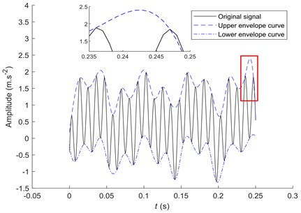
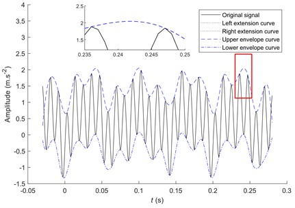
Fig. 2The EMD decomposition after extension

The solid line in Fig. 1 is the original signal given by Eq. (2) in the interval [0, 0.25] s. The dashed and dash-dotted lines are the upper and lower envelopes of the original signal, respectively. Fig. 1 shows that the envelope curve has a large oscillation at the right end of the signal. The envelope line and data sequence intersect in the local amplification diagram in Fig. 1, which cannot contain all the data. Hence, it cannot ensure the correct decomposition of the signal. The standard deviation of the upper envelope without extension is 0.4022 and the peak index is 1.5517.

To prevent the occurrence of this phenomenon, it is necessary to extend the waveform at both ends of the signal and increase the length of the waveform to suppress the endpoint effect [24].

Fig. 2 extends the signal length to [–0.03, 0.28] s, where the dotted line is the signal extended on both sides. The standard deviation of the envelope is 0.3959 and the peak index is 1.3828. Compared to the local amplification diagram of Figs. 1-2, the waveform after extension is smoother. It can reduce the possibility of sharp changes at the end. Therefore, the signal extension significantly inhibits the endpoint effect. There is no irregular oscillation of the fitting curve, and the data are not included.

In summary, a signal cannot be accurately decomposed by relying only on its extreme points to suppress the endpoint effect. It is necessary to extend the two ends of the signal and combine them with the change trend of the original signal waveform. One maximum and one minimum values are added at both ends of the signal [25]. The endpoint effect is moved outward to reduce the decomposition error of the original signal.

3. Relationship between slope integral and waveform

The peak solution [26, 27] is the limit state that reflects the amplitude fluctuation within the local time-length. It extracts the adjacent maximum (minimum) of the signal waveform to form a peak decomposition diagram and is effectively applied in the time-frequency domain of nonlinear signals. The adjacent maximum (minimum) is of great significance for fault feature extraction.

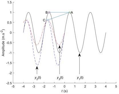
As shown in Fig. 3, points $A$ and $B$ are two adjacent maximum points on a sinusoidal signal. The slope of line $l_{AB}$ is zero. When point $C$ on the point line is a point on the signal, the slope of line $l_{AC}$ is not zero. When the signal waveform changes suddenly, the slope between adjacent maximum points changes [28]. That is, the slope is an important indicator of waveform change trend. Fig. 3 shows that although the signal $y_2\left(t\right)$ and $y_3\left(t\right)$ intersect at the maximum point $C$, the signal waveforms and amplitudes of the two are different. $E_{y_2}$ denotes the integral of the line $l_{AC}$ and signal $y_2\left(t\right)$ in the range of $[t_C,t_A]$, that is, the vibration energy in the interval. $E_{y_3}$ denotes the integral of the line $l_{AC}$ and signal $y_3\left(t\right)$ in the range of $[t_C,t_A]$. The randomness of the signal is visible in Fig.3. It implies that $E_{y_2}\ne E_{y_3}$. Therefore, the vibration energy reflects the amplitude and waveform shape. Through the above analysis, it is evident that slope and vibration energy are important indices of waveform, and the key references for waveform extension.

Fig. 3Relationship between vibration energy and slope

4. SIEMD algorithm design

To overcome the above mentioned shortcomings and improve the matching degree of the extended signal, the SIEMD method is proposed in this study. This method is based on the segmentation baseline and motion energy in the signal extreme point interval. It matches the interval and extracts the extension characteristics. Finally, it fits the optimal extension curve using motion energy as the iterative termination condition. Assuming that the first extreme value of the signal is the maximum value, the implementation steps are as follows.

Find the extreme value: The extreme points of the original signal are calculated. The set of local maximum points is $E_{\mathrm{m}\mathrm{a}\mathrm{x}}$, and the corresponding time set is $t_{\mathrm{m}\mathrm{a}\mathrm{x}}$. The set of local minimum points is $E_{\mathrm{m}\mathrm{i}\mathrm{n}}$, and the corresponding time set is $t_{\mathrm{m}\mathrm{i}\mathrm{n}}$.

Seek slope and motion energy of the extreme point interval. The slope $k_1$ (Eq. (3)) and segmentation baseline $y_1$ (Eq. (4)) of points ($t_{\mathrm{m}\mathrm{a}\mathrm{x}}^1$, $E_{\mathrm{m}\mathrm{a}\mathrm{x}}^1$) and ($t_{\mathrm{m}\mathrm{a}\mathrm{x}}^2$, $E_{\mathrm{m}\mathrm{a}\mathrm{x}}^2$) are calculated. The function of fitting curve $E_{\mathrm{m}\mathrm{a}\mathrm{x}}^1{E}_{\mathrm{m}\mathrm{i}\mathrm{n}}^1{E}_{\mathrm{m}\mathrm{a}\mathrm{x}}^2$ with least squares polynomial is $s_1$. The motion energy $S_1$ surrounded by the segmentation baseline $y_1$ and curve $s_1$ is calculated (Eq. (5)). The order $m_1$ needs to be determined for least squares polynomial fitting. The symbol $len$ represents the length of set $E_{\mathrm{m}\mathrm{a}\mathrm{x}}$. To ensure the fitting accuracy, $m_1=6$.

The slope calculation equation is as follows:

The calculation equation of segmentation baseline is as follows:

The motion energy calculation equation is as follows:

Select the optimal matching curve $s_j$ with $s_1$ according to the comprehensive index $I_j$. The slope set is $k=[k_1,k_2,\cdots ,k_{len-1}]$, and the motion energy set is $S=[S_1,S_2,\cdots ,S_{len-1}]$. The comprehensive index is $I_i=|S_1-S_i|+|k_1-k_i|$($1<j\le len-1$). Considering the sampling frequency, $|S_1-S_i|$ and $|k_1-k_i|$ are not in one order of magnitude. Therefore, the comprehensive indicators are improved as: $I_i=A\mathrm{*}|S_1-S_i|+B\mathrm{*}|k_1-k_i|$. In the equation, $A$ and $B$ represent the proportion of slope and integral differences, respectively. They can be adjusted according to practical application scenarios. In this study, $A=10^3$, $B=10^{-2}$. The set $I=[I_1,I_2,\cdots ,I_{len-1}]$ is obtained by the slope set and the motion energy set. The interval corresponding to the minimum comprehensive index $I_j$($1<j\le len-1$) is selected. Subsequently, the curve $s_j$ of the interval is determined to be the most similar to the curve $s_1$.

Extract the extension information. According to the step 3 , the values of slope $k_{j-1}$ and motion energy $S_{j-1}$ from $E_{\mathrm{m}\mathrm{a}\mathrm{x}}^{j-1}$ to $E_{\mathrm{m}\mathrm{a}\mathrm{x}}^j$ are calculated, the data length of the interval $n$ is counted, and position relationship $p_{j-1}$ between the minimum point $t_{\mathrm{m}\mathrm{i}\mathrm{n}}^{j-1}$ and maximum point $t_{\mathrm{m}\mathrm{a}\mathrm{x}}^j$ in the interval is stored.

Extension waveform. Segmentation baseline $y_0$ is based on the values of $k_{j-1}$, $t_{\mathrm{m}\mathrm{a}\mathrm{x}}^1$ and $E_{\mathrm{m}\mathrm{a}\mathrm{x}}^1$. Maximum $E_{\mathrm{m}\mathrm{a}\mathrm{x}}^0$ and minimum $E_{\mathrm{m}\mathrm{i}\mathrm{n}}^0$ of extension interval are calculated according to the data number $n$, the baseline $y_0$ and position relationship $p_{j-1}$. The least square polynomial fitting curve $s_0$ is obtained by synthesizing the data of extreme points and endpoints of extension. The order of the least square method is $m_2=3$. The motion energy $S_0$ is calculated (Eq. (5)). When the termination condition $A\mathrm{*}|S_0-S_{j-1}|<0.1$ is satisfied, the output curve $s_0$ is the left extension waveform. Otherwise, let $m_2=m_2+1$, repeat $s_0$ and compare the size of $A\mathrm{*}|S_0-S_{j-1}|$ and 0.1 in each case until the termination condition is satisfied.

The left extension is completed. The extension process is shown in Fig. 4(a). If the first extreme value is the minimum value, it is similar to the above mentioned method. Thus, the right endpoint extension curve can also be derived. The new signal is obtained and IMFs are obtained by the EMD decomposition.

Fig. 4Slope integral extension diagram

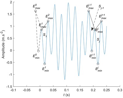
a) The SIEMD diagram

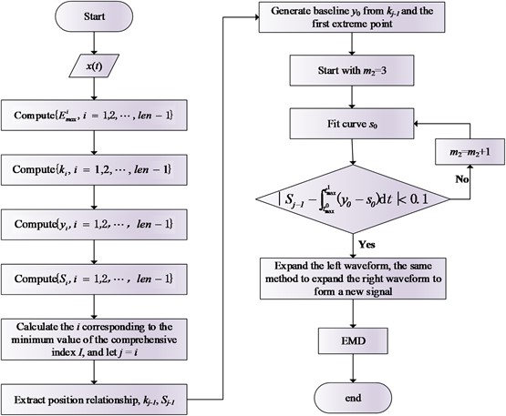
b) The SIEMD flow chart

5. Simulated signal analysis

To verify the feasibility of the SIEMD method proposed in this study, the simulation signal is decomposed and compared with the EMD and the mirror extension of the EMD. The simulation signal expressions used are as follows:

The sampling frequency is 1000 Hz, the variable range is $t\in$ [0, 0.5] s, and the original signal waveforms are shown in Fig. 5.

Fig. 5Original signal and its component signals

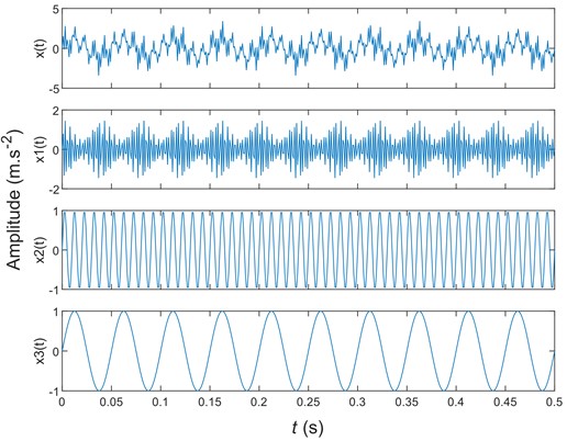
Fig. 6The EMD decomposition without endpoint processing

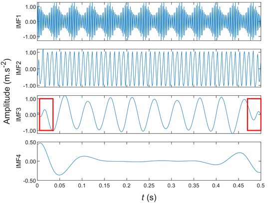
Figs. 6-8 are the signals of Eq. (6) obtained by non-extension EMD, mirror extension EMD, and SIEMD, respectively. Due to the decomposition of more components, the first four are selected here for display. Compared with the intermediate waveform of IMF3 component, there is a large amplitude error in Fig. 6 and Fig. 7, and there is a serious endpoint effect. The waveform at the red mark in Fig. 8 is more consistent with the whole, which greatly suppresses the endpoint effect. Compared with the IMF4 component, the amplitude obtained by the SIEMD method is smaller than other methods, showing a smaller decomposition error. Thus, the mirror extension method cannot effectively suppress the endpoint effect in Eq. (7):

Fig. 7Mirror extension of the EMD decomposition

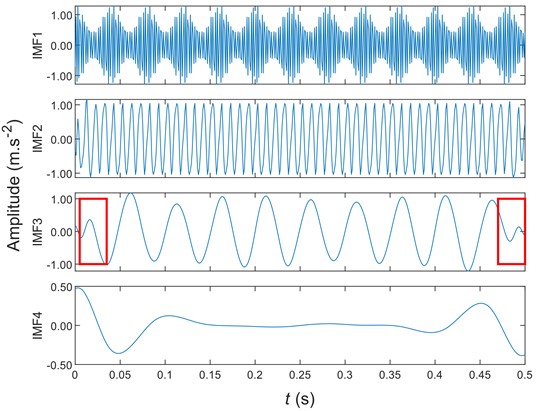
Fig. 8The SIEMD decomposition

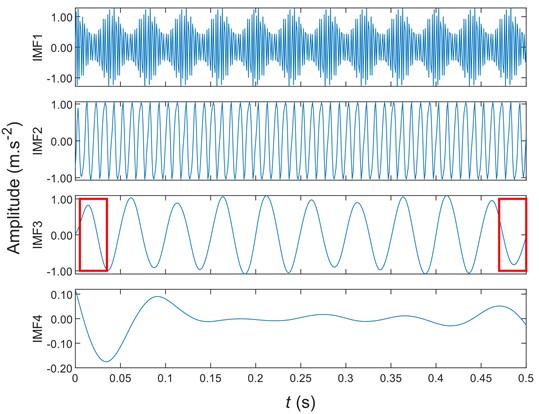
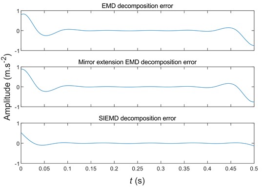
Fig. 9 is based on Eq. (7) to calculate the error between the original signal $x\left(t\right)$ and the first three components obtained after the EMD decomposition. Fig. 9 shows that compared with the EMD decomposition and the mirror EMD decomposition, the SIEMD decomposition error is negligible. There are no significant oscillations at both ends. It shows that the SIEM significantly suppresses the endpoint effect.

The following two indices are used to evaluate the effect of the endpoint-effect processing method.

1) The correlation coefficient $\rho$ between each component after the EMD decomposition and corresponding component of the original signal are calculated to evaluate the effect of endpoint suppression:

where $\mathrm{c}\mathrm{o}\mathrm{v}(\cdot )$, $\sigma (\cdot )$, $IM{F}_i\left(t\right)$ and $x_i\left(t\right)$ represent the covariance, the variance, the $i$th IMF component of the original signal after the EMD decomposition, and the $i$th corresponding component of the original signal, respectively. A value of ${\rho }_i\left(x_i\right(t),IM{F}_i(t\left)\right)$ closer to 1 indicates better endpoint suppression.

2) The average relative error between components after the EMD decomposition and corresponding components of the original signal are calculated:

where $N$, $IM{F}_i\left(k\right)$, and $x_i\left(k\right)$ represent the number of signal acquisition, and $k$th data in the $i$th corresponding component of the original signal, respectively. The closer is $error\_IM{F}_i$ to 0, the smaller is the error between the decomposed and original signals.

Fig. 9The EMD, mirror EMD, and SIEMD decomposition error

According to Eqs. (5-6), the evaluation indexes of non-extension, mirror extension, and SIEMD are calculated. The results are listed in Table 2.

By the SIEMD method, the values of ${\rho }_1\left(x_1\right(t),IM{F}_1(t\left)\right)$, ${\rho }_2\left(x_2\right(t),IM{F}_2(t\left)\right)$ and ${\rho }_3\left(x_3\right(t),IM{F}_3(t\left)\right)$ are 0.9720, 0.9505 and 0.9915, respectively, which are closer to 1. The results presented in Table 1 reveal that the correlation coefficient of the SIEMD method is greater than the EMD decomposition of non-extension and mirror extension. The average relative error of the EMD decomposition by the SIEMD method is less than that of the EMD decomposition without extension and mirror extension. By the SIEMD method, the value of $error\_IM{F}_i$ is closer to 0. This indicates the effectiveness and feasibility of the SIEMD method.

6. Actual signal analysis

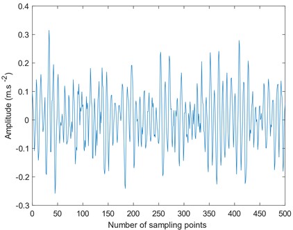
To further verify the effectiveness of the extension method, a nonlinear and non-stationary bearing fault signal is analyzed. The fault signal is collected from a test rig containing faulty bearings. The test bench shown in Fig. 10(a) is composed of motor, drive shaft, test rolling bearing and signal acquisition system. A crack with a width of about 0.2 mm is cut at the inner ring (see Fig. 10(b)) of the bearing by wire cut electrical discharge machining. The motor speed is 1940 r/min, and the theoretical bearing inner ring fault frequency is 159.96 Hz. The fault signal is shown in Fig. 11.

Fig. 10Fault signal acquisition equipment

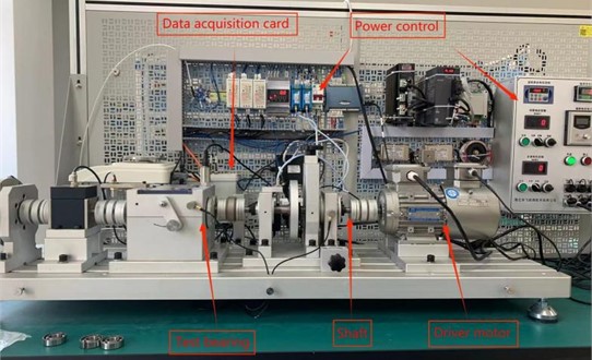
a) The test rig

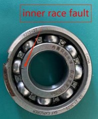
b) The test bearing

Fig. 11Fault signal of bearing inner ring

The fault signals are processed using non-extension EMD, mirror extension EMD, and SIEMD. The components after decomposition are as follows.

Fig. 12The EMD decomposition

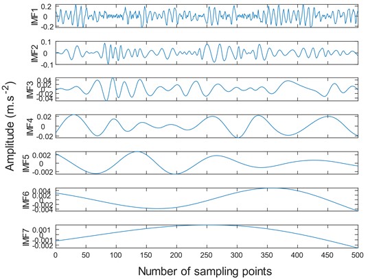
a) The EMD decomposition of fault signals

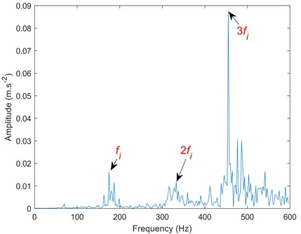
b) Spectrum corresponding to IMF₁ component

Fig. 13Mirror extension EMD decomposition

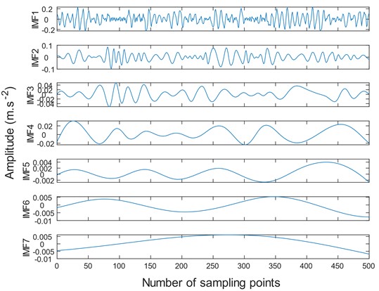
a) Mirror extension EMD decomposition of fault signal

b) Spectrum corresponding to IMF₁ component

Fig. 14The SIEMD decomposition

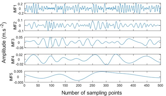
a) The EMD decomposition of fault signal by SIEMD

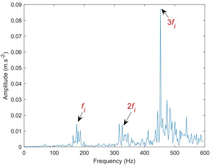
b) Spectrum corresponding to IMF₁ component

Compared to Figs. 12-14, the traditional EMD and mirror extended EMD decomposed the signal into seven components. Whereas the SIEMD method decomposed the signal into only five IMF components. Excessive components will reduce the signal fault extraction rate and may cause information redundancy and dimension disaster. Comparing the spectrum, it can be seen that the SIEMD method is more prominent at the second harmonic frequency, which is convenient for accurately judging the fault type.

The data in Table 3 are the correlation coefficients between the first four components of the bearing inner ring fault signal and EMD, mirror EMD, and SIEMD and the fault signal. According to the data in Table 3, the similarity between IMF₁ component and fault signal is the highest, while the similarity between component IMF₄ and fault signal is the lowest, indicating that the similarity between each component and fault signal is decreasing, that is, the first component obtained has more fault information and has the highest correlation with fault signal. Compared with EMD [22], mirror EMD [16] and SIEMD, the similarity between the component obtained by the SIEMD method and the fault signal is the highest, reaching 92.03 %, which has greater advantages than the other two methods. If the correlation coefficient between the two is large, it is judged to be an effective IMF component. If the correlation coefficient between the two is small, it is judged to be a false component. The double fault frequency at Fig. 14(b) is more prominent than other methods. Therefore, compared with the mirror extension method, SIEMD can weaken the influence of the endpoint effect to a greater extent and extract the signal fault signal faster.

7. Conclusions

Here, the SIEMD method is proposed to suppress the end effect of the EMD. Considering the slope of signal extremum and motion energy, this method uses the least squares-polynomial fitting to extend the waveform of fault signal.

Compared with the traditional EMD [22] and mirror EMD [16], the proposed SIEMD decomposition method extracts less IMF components, higher correlation coefficient, and smaller relative error. It is beneficial for the extraction of fault feature information.

The SIEMD method overcomes the shortcomings of the original signal waveform and can effectively suppress the endpoint effect generated by the EMD. Therefore, the decomposition accuracy of this method is superior to that of the EMD.

The subsequent work will study the influence of signal waveform on signal decomposition and the significance of signal energy to signal decomposition, and propose a new decomposition method on this basis.