Energy analysis of living stumps slope based on Hilbert-Huang Transform and marginal spectrum

1. Introduction

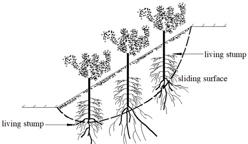
Although the traditional slope protection structures (such as concrete retaining walls, concrete anti-slide piles, and anchor bodies) can effectively improve slope stability, they are costly, and are prone to weathering of the slope and aging of concrete materials, resulting in the decrease of structural strength and the significant weakening of protective effect, which in turn causes slope erosion and soil erosion, thereby damaging the ecological environment [1]. The plant ecological slope protection technology can effectively improve the stability of slope through the shallow root reinforcement and deep root anchorage of plant roots [2-4]. In addition, the technology reduces soil moisture content and pore water pressure through the absorption and transpiration of plants [5], thereby improving the shear strength of the soil. Moreover, with the increase of time, the plant roots continue to extend deep into the soil, which is helpful to control the shallow sliding and collapse of the slope [6], making it become an ecological protection technology with “vitality” [7]. However, the traditional plant slope protection technology is mainly aimed at the prevention and control of shallow landslides [8], and cannot effectively reinforce deep landslides (2-5 m). Therefore, the research group proposed a living stumps slope support structure, which implants the vigorous seedlings (elm trees, etc.) with strong vitality into the deep soil layer or cuts their branches into the deep soil layer. The roots grow outward with time, forming a root-soil complex in the deep soil layer, thus playing a role in slope reinforcement, as shown in Fig. 1. The living stumps are an environmentally friendly form of slope protection with the potential to prevent deep-seated landslides. The existing research results indicate that living stumps make the maximum shear stress zone of the slope move to the deep soil [9], and have a good supporting effect on the deep landslide [10]. The safety factor of slopes supported by living stumps is increased by 30-50 % compared to the original slopes under static action [11].

As we all know, earthquakes are an important cause of slope instability [12]. The presence of living stumps alters the waveform of seismic waves and the propagation characteristics of seismic waves within the slope’s rock and soil mass, which makes the seismic interaction mechanism between living stumps and rock and soil very complicated. R. Sonnenberg [13] carried out a series of centrifuge model tests to reveal the failure mechanism of clay slope reinforced by model roots, and pointed out the contribution of lateral roots in slope reinforcement; Liang [14] used 3D printing technology to create model roots and conducted centrifuge model tests to study the response of vegetated slopes during earthquakes. It was found that plant roots reduced the settlement of the slope top by 67 % during the sliding process under the action of earthquakes; Niu [15] based on a shallow sliding failure model, derived the dimensionless stability factors for slopes with and without vegetation protection using limit analysis methods. It was found that the safety factor calculated by the infinite slope model had been increasingly underestimated. The above research on the seismic dynamic response of the model root supported slopes mainly focuses on the traditional mechanical analysis, and mostly stays in the time domain and frequency domain, without fully considering the influence of energy on their dynamic response. Energy is an important factor to induce the dynamic response of slope [16]. Therefore, studying the dynamic response of root-supported slopes from an energy perspective is of significant importance. In addition, domestic and foreign scholars commonly use Fourier transform [17] and wavelet transform [18] to process the acceleration signals of each monitoring point under earthquakes. However, Fourier transform is suitable for linear stationary signals, which can only provide the spectral information of the signal and lacks the ability of time domain localization [19]. It is difficult for wavelet transform to analyze signals with transient behavior, and the effectiveness of its analysis results depends on the selection of wavelet basis function [20]. In contrast, Hilbert-Huang transform (HHT) has good time-frequency resolution, more accurately reflects the time-frequency variation characteristics of the signal, and fully demonstrates the energy distribution characteristics of seismic waves in the time-frequency domain. And it has high adaptability to nonlinear and non-stationary signals [21]. At the same time, Hilbert-Huang transform decomposes the signal into multiple intrinsic mode functions (IMFs) by empirical mode decomposition (EMD), and calculates the instantaneous energy of each IMF and accumulates to obtain the total Hilbert energy of the seismic signal [22]. The energy of traditional physics refers to the kinetic energy, potential energy or thermal energy of an object or system, which follows the law of conservation of energy. In contrast, seismic Hilbert energy is a representation of energy derived from Hilbert-Huang Transform for time-frequency analysis of signals, aimed at revealing the energy distribution characteristics of nonlinear and non-stationary seismic signals in the time-frequency domain.

Fig. 1Living stumps for slope stabilization

A large-scale shaking table test on a slope with living stumps was conducted, in which an elm tree root model was constructed using 3D printing technology. The acceleration data collected from within the slope under seismic loading were analyzed using the Hilbert-Huang Transform (HHT), enabling quantitative assessment of time-frequency characteristics and energy distribution changes in the nonlinear system. This approach revealed the high-frequency dynamic response features and detailed response mechanisms of slopes with living stumps under earthquake loading. The findings provide a novel analytical framework for evaluating the reinforcing effects of root systems on slopes during earthquakes, aiming to offer theoretical support for the seismic design of slopes incorporating living stumps.

2. Shaking table test design

2.1. Experimental equipment system and its main parameters

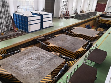
The shaking table model test was completed on the multifunctional shaking table system at the National Engineering Laboratory for High-Speed Railway Construction Technology of Central South University, as shown in Fig. 2. The main technical parameters of the shaking table system are the table size of 4 m× 4 m; the maximum load is 30 tons, rated velocities of ±1000 mm/s in $X$, $Y$, $Z$ directions; the rated accelerations of ±1.0 g in $X$, $Y$ directions, and ±2.0 g in $Z$ direction; and the operating frequency range is 0.1-50 Hz. The data acquisition instrument of the model test is the IMC-CRFX-400 dynamic data acquisition system.

Fig. 2Shaking table test

2.2. Model design

2.2.1. Similarity relationships

The reliability of shaking table model tests lies in whether the model can accurately reflect the dynamic response of the prototype structure. In this study, dimensional analysis based on the Buckingham $\pi$ theorem [23] was employed to derive the similarity constants for all physical quantities involved in the model test. Upon analysis and organization, it was identified that the shaking table model test of slopes with living stumps involved 14 physical quantities, as shown in Table 1.

Table 1Physical quantities of model test

Serial number	Physical quantity	Serial number	Physical quantity
1	Length / $L$	8	Acceleration / $a$
2	Density / $\rho$	9	Time / $t$
3	Elastic modulus / $E$	10	Stress / $\sigma$
4	Poisson ratio / $\mu$	11	Strain / $\epsilon$
5	Gravity / $\gamma$	12	Velocity / $v$
6	Force of cohesion / $c$	13	Displacement / $u$
7	Angle of internal friction / $\phi$	14	Vibration frequency / $\omega$

Based on the 14 physical quantities listed in the table, the general expression of the similarity criteria, Eq. (1) can be derived:

1

$\begin{array}{r}\pi =[L{]}^{a_1}\cdot [\rho {]}^{a_2}\cdot [E{]}^{a_3}\cdot [\mu {]}^{a_4}\cdot [\gamma {]}^{a_5}\cdot [c{]}^{a_6}\cdot [\phi {]}^{a_7}\cdot \\ [a{]}^{a_8}\cdot [t{]}^{a_9}\cdot [\sigma {]}^{a_{10}}\cdot [\epsilon {]}^{a_{11}}\cdot [v{]}^{a_{12}}\cdot [u{]}^{a_{13}}\cdot [\omega {]}^{a_{14}}.\end{array}$

Furthermore, by substituting the dimensional expressions of each physical quantity from Table 1 into Eq. (1) and applying the principle of dimensional consistency, the similarity criteria expressed as Eq. (2) can be obtained:

2

$\begin{array}{c}{M}^{0}L{T}^0=M^{\left(a_2+a_3+a_5+a_6+a_{10}\right)}\cdot L^{\left(a_{`}-3a_2-a_3-2a_5-a_6+a_8-a_{10}+a_{12}\right)}\end{array}$
$\bullet T^{\left(-2a_3-2a_5-2a_6-2a_8+a_9-2a_{10}-a_{12}-a_{14}\right)}.$

According to the geometric size, density and acceleration similarity ratio selected by IAI [24] and Yang [25, 26] as the main control parameters, the similarity constants are determined to be $C_1=\text{7}$, $C_{\rho }=\text{1}$ and $C_a=\text{1}$. The other primary similarity constants were determined based on the above derivation, as presented in Table 2 [28].

Table 2Primary similitude coefficients of model

Physical quantity	Similarity relation	Similarity constant
Length / $L$	$C_l$	7
Density / $\rho$	$C_{\rho }=1$	1
Acceleration / $a$	$C_a=1$	1
Gravity / $\gamma$	$C_{\gamma }=C_{\rho }$	1
Velocity / $v$	$C_v=C_l^{0.5}$	2.65
Displacement / $u$	$C_u=C_l$	7
Time / $t$	$C_t=C_l^{0.5}$	2.65
Cohesion / $c$	$C_c=C_l\bullet C_{\rho }$	7
Internal friction angle / $\phi$	$C_{\varphi }=1$	1
Poisson’s ratio / $\mu$	$C_{\mu }=1$	1
Stress / $\sigma$	$C_{\sigma }=C_l\bullet C_{\rho }$	7
Strain / $\epsilon$	$C_{\epsilon }=1$	1
Vibration frequency / $\omega$	$C_{\omega }=1$	1
Elastic modulus / $E$	$C_E=C_l\bullet C_{\rho }$	7

2.2.2. Model box design and boundary treatment

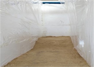
The rigid model box was used in the test [27, 28], and the internal clearance size was 350 cm×150 cm×210 cm (length×width×height). In addition, the diagonal braces were welded at the bottom of the model box to enhance stability, and the bolt holes were pre-drilled in the bottom plate of the model box for fixation purposes. In order to reduce the “model box effect” [29], the boundaries of the model box were treated accordingly [30]. To increase bottom friction and prevent relative sliding between the model and the model box, a layer of 4cm gravel was laid at the bottom of the model box, followed by a layer of fine sand to fill the gaps. In order to weaken the reflection of seismic waves in the model box, a 5 cm thick polyethylene foam board was pasted on the three sides of the inner wall of the model box. In order to reduce the friction between the model and the boundary, a polyvinyl chloride film was pasted on the foam board. The boundary treatment is shown in Fig. 3.

Fig. 3Boundary processing

2.2.3. Experimental materials

A 30 cm-thick composite material was placed at the bottom of the model box to simulate the bedrock of the slope. The composite consisted of barite powder, quartz sand, and lithium-based lubricating grease, mixed in a ratio of 10:5:1. The main body of the slope was constructed using cohesive soil type [31], with the particle size of the test soil material controlled to not exceed 1 cm. Specific material parameters are provided in Table 3.

Table 3Material physical and mechanical parameters

Material type	Density / $\rho$ (g/cm3)	Poisson’s ratio / $\mu$	Internal friction angle / $\phi$ (°)
Cohesive soil	1.837	0.3	17
Bedrock	2.202	0.38	22.5

Plant root systems were classified into six types by Yen [32] and Gray [33]. Among these, the root system with a well-developed primary root that grows vertically downward, and secondary roots concentrated in the upper 1/3 region of the primary root extending towards the periphery, is categorized as the “VH” type. Furthermore, the shear resistance of living stumps is primarily determined by the length of the primary root, while the anchoring effectiveness is influenced by the orientation and lateral expansion width of the secondary roots. Therefore, the “VH” type elm root system was selected as the prototype for the living stumps.

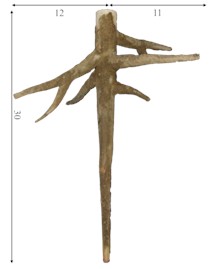
Acrylonitrile-butadiene-styrene (ABS) material has been proven to effectively simulate the strength and stiffness of roots and can be precisely constructed into root system models in scale through 3D printing technology [34, 35]. In the experiment, based on the growth patterns and three-dimensional morphology of the elm root system, it was simplified into one primary root and five secondary roots. The cross-sections of both the primary and secondary roots are circular, with cross-sectional areas decreasing linearly from the proximal to the distal ends. The living stump model was fabricated using ABS material and 3D printing technology at a geometric similarity ratio of 1:7. Epoxy resin was used to uniformly adhere a layer of quartz sand onto the surface of the living stump model to increase the friction between the model and the soil. The simulated main root length of real elm roots was 2.1 m, and the lateral root lengths from top to bottom were 0.77 m, 0.84 cm, 0.77 cm, 0.595 cm and 0.315 cm, respectively. The ABS material and the living stump model are shown in Fig. 4 and Fig. 5, respectively.

Rectangular distribution is the best mode to improve the stability of living stumps slope[36]. For this experiment, 9 living stump models were constructed and arranged in a 3-row by 3-column configuration within the slope. The center of the living stumps matrix was positioned along the central axis of the slope surface, with a horizontal distance of 38 cm and a vertical distance of 30 cm between adjacent stumps.

Fig. 4ABS material pictures

Fig. 53D printed model of a living stump (Unit: cm)

2.3. Sensor arrangement

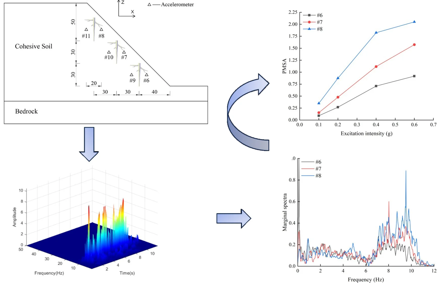
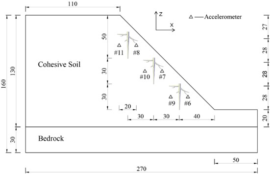
The acceleration was measured using a uniaxial accelerometer model 1221L-002, with a range of ±20 m/s² and a sensitivity of 2000 mv/g. The accelerometer measurement points were arranged as shown in Fig. 6, and the accelerometer measuring points were numbered A6-A11 (A0 was located on the shaking table to test the seismic wave input). Considering that the loading of seismic waves was bidirectional, sensors monitoring dynamic responses in both the horizontal ($x$-axis) and vertical ($z$-axis) directions were placed at each measurement point. All acceleration measuring points were arranged on the inside and outside of the middle column of living stumps, and were located on the central axis. The living stumps were sequentially named from the slope toe to the crest as Living Stump I, Living Stump II, and Living Stump III.

Fig. 6Layout of accelerometer measuring points (Unit: cm)

2.4. Seismic wave excitation scheme

Bidirectional excitation waves, including the Kobe wave (K-XZ) and the Darya artificial wave (DR-XZ), were selected as input motions with a time compression ratio of 2.65. Fig. 7 and Fig. 8 show the time-history curves and Fourier spectra of the input waves at a peak horizontal acceleration of 0.4 g. According to the seismic design code [37], the peak acceleration of the vertical seismic wave is 2/3 of the peak horizontal acceleration. The loading scheme for the test is shown in Table 4.

Fig. 7Acceleration time-history curve (0.4 g)

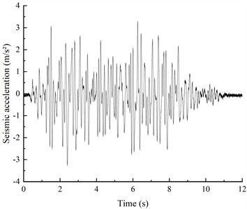
a) K-XZ

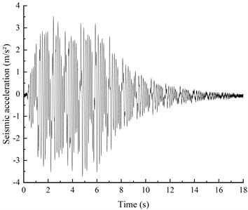
b) DR-XZ

Fig. 8Fourier spectrum curves (0.4 g)

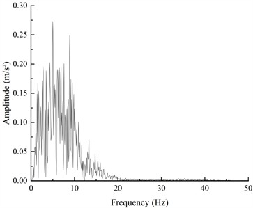
a) K-XZ

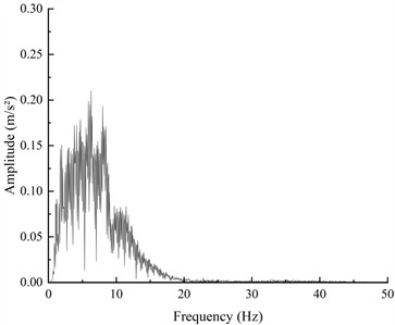
b) DR-XZ

Table 4Loading sequences of the test

Serial number	Seismic wav	Peak acceleration /g
		X	Z
1	WN-1	–	–
2	DR-XZ	0.1	0.067
3	K-XZ	0.1	0.067
4	WN-2	-	-
5	DR-XZ	0.2	0.133
6	K-XZ	0.2	0.133
7	WN-3	–	–
8	DR-XZ	0.4	0.267
9	K-XZ	0.4	0.267
10	WN-4	–	–
11	DR-XZ	0.6	0.4
12	K-XZ	0.6	0.4
13	WN-5	–	–

3. Seismic response analysis of internal acceleration of living stumps

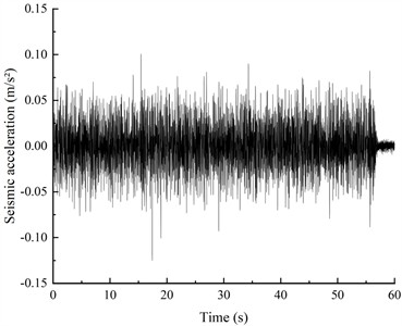
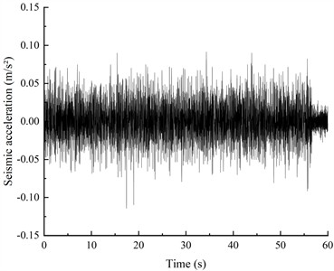
To verify the consistency of seismic waves during input and output, an accelerometer was placed at point A0 on the shaking table surface. Taking the excitation intensity of 0.4g for K-XZ as an example, Fig. 9(a) shows the acceleration time-history curve recorded at point A0, while Fig. 9(b) presents the acceleration time-history curve input into the model.

Fig. 9Verification of K-XZ input at 0.4g excitation intensity

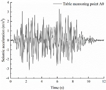
a) Table measuring point A0

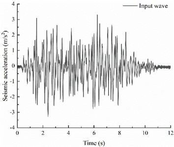
b) Input wave

As shown in Fig. 9(a) and Fig. 9(b), there was no energy loss during the input process of the 0.4 g K-XZ wave, indicating that the input and output seismic waves remained consistent, thereby ensuring the reliability of the experimental data.

In order to detect the dynamic characteristics of the slope model, a 60s white noise with a peak acceleration of 0.08 g was input before and after the test [38], and when the excitation acceleration peak value changed (denoted as WN-1 to WN-5). After the model was input with white noise WN-1 and WN-5, the horizontal acceleration time history curve from A8 inside the living stumps slope model (as shown in Fig. 10) indicates that the changes in the horizontal acceleration time history curve are minimal, and the internal structural damage of the model can be ignored.

Fig. 10Presents the time history curve of horizontal acceleration at point A5 after white noise scanning at different stages

a) WN-1

b) WN-5

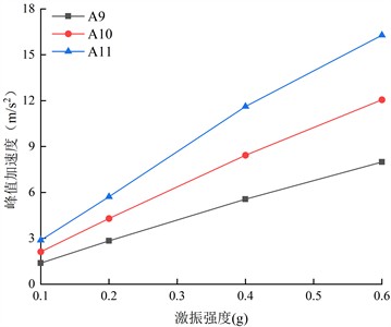
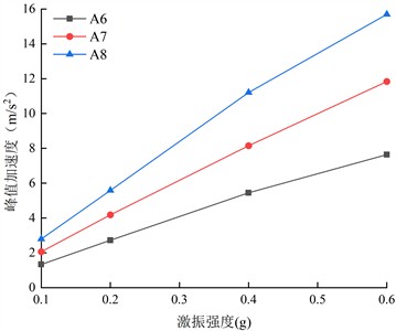
The bidirectional loading of seismic waves caused the acceleration of the living stumps slope in both horizontal and vertical directions. The acceleration response in the horizontal direction is significantly higher than that in the vertical direction, the analysis focuses on the horizontal peak acceleration [39]. Fig. 11 shows the horizontal peak accelerations at various monitoring points inside the living stumps slope under different excitation intensities of K-XZ and DR-XZ. As shown in Fig. 11, under the action of K-XZ with an excitation intensity of 0.2 g, the horizontal peak acceleration values at the monitoring points on the inner side of the living stumps increase from 2.799 to 5.112 with the elevation. The values at the monitoring points on the outer side (A6 to A8) increase from 2.768 to 5.053, showing a significant acceleration amplification effect. In addition, under the other three excitation intensities, the horizontal peak accelerations on both sides of the living stumps inside the slope also gradually increase with elevation. Further analysis indicates that as the excitation intensity increases, the horizontal peak accelerations at all monitoring points on both sides of the living stumps inside the slope also gradually increase. Taking the monitoring point A8 as an example, as the excitation intensity increased from 0.1 g to 0.6 g, the horizontal peak acceleration value at A8 increased from 2.549 to 14.344. This indicates that in the living stumps slope, the horizontal peak accelerations of the monitoring points on both sides of the living stumps are positively correlated with excitation intensity and elevation.

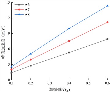
Fig. 12 shows the horizontal peak accelerations of the monitoring points on both sides of the living stumps inside the slope under different excitation intensities of DR-XZ. Comparing Fig. 11 with Fig. 12, it is evident that the horizontal peak acceleration variation patterns of the monitoring points on both the inside and outside of the living stumps are similar under DR-XZ and K-XZ actions, increasing with elevation and excitation intensity. Meanwhile, the acceleration time-history variation patterns at the monitoring points on both sides are also similar, positively correlated with excitation intensity and elevation. This indicates that the type of seismic wave mainly affects the magnitude of the acceleration, but has little impact on the variation pattern of the horizontal peak acceleration.

Fig. 11Horizontal peak acceleration on both sides of the living stumps inside the slope under different excitation intensity K-XZ

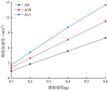
a) Inside

b) Outside

Fig. 12The Horizontal peak acceleration on both sides of the living stumps inside the slope under different excitation intensity DR-XZ

a) Inside

b) Outside

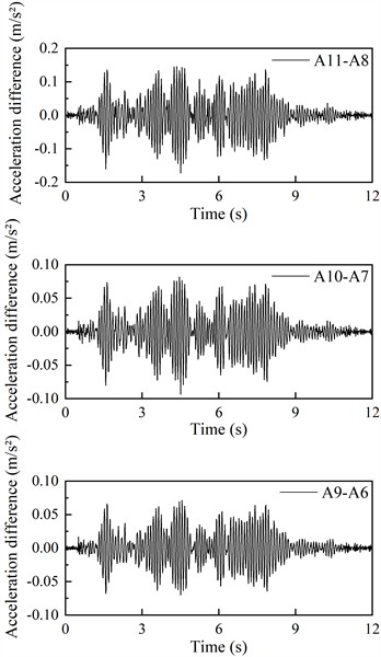
In the shaking table test, the horizontal acceleration time histories of the monitoring points on both sides of the living stumps inside the slope were obtained. Comparison of the acceleration time histories at both sides reveals that, at the same time, the directions of the accelerations are consistent. The horizontal acceleration time history of the monitoring points on the inner side of the living stumps is subtracted from the horizontal acceleration time history of the monitoring points on the outer side of the living stumps, and the horizontal acceleration time history difference of the monitoring points on both sides of the living stumps is obtained. Due to space constraints, only the differences in acceleration time histories at the monitoring points on both sides of the living stumps under 0.4 g excitation intensity for K-XZ and DR-XZ actions are presented (see Fig. 13). As shown in Fig. 13(a), under 0.4g K-XZ action, the difference in horizontal acceleration of the monitoring points on both sides of the living stumps is greatest at the top of the slope, followed by the middle of the slope, and smallest at the base. This indicates that the absolute value of the horizontal acceleration difference between the monitoring points on both sides of the living stumps is positively correlated with elevation. This is particularly notable in terms of horizontal peak acceleration, where the difference in horizontal peak acceleration between the monitoring points increases from 0.055 to 0.125 with rising elevation. In addition, with the increase of the excitation intensity, the absolute value of the horizontal acceleration time history difference of the monitoring points on both sides of the living stumps also increases gradually. For example, when the excitation intensity increases from 0.1 g to 0.6 g, the difference value of the horizontal peak acceleration of the monitoring points on both sides of the slope top living stumps increases from 0.023 to 0.162.

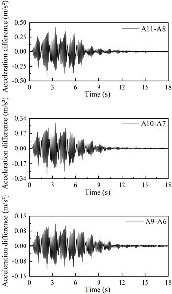
Fig. 13(b) shows the horizontal acceleration time history difference of the monitoring points on both sides of the living stumps under the action of 0.4 g DR-XZ. Comparing Fig. 13(a) and Fig. 13(b), it can be seen that the variation pattern of horizontal acceleration difference under DR-XZ action is similar to that under K-XZ action, and its absolute value is positively correlated with elevation and excitation intensity. However, there is a significant difference between the two values. The absolute value of the horizontal acceleration difference under DR-XZ is greater than that under K-XZ. This indicates that the type of seismic wave has little effect on the variation pattern of the horizontal acceleration difference between the monitoring points on both sides of the living stumps, mainly affecting its magnitude. Furthermore, the difference of horizontal acceleration time history on both sides of the living stumps reveals the difference of seismic dynamic response on both sides. The dynamic response on the inner side of the living stumps is significantly larger than that on the outer side, and this difference increases with the increase of excitation intensity and elevation. Therefore, it is great significance to explore the causes of the dynamic response differences on both sides of the living stumps in the slope. The following text will analyze the causes of these differences in dynamic responses based on Hilbert-Huang Transform and marginal spectra, focusing on energy distribution and time-frequency characteristics.

Fig. 13The horizontal acceleration difference on both sides of the living stumps inside the slope under different input waves with excitation intensity of 0.4 g

a) K-XZ

b) DR-XZ

4. Analysis of seismic Hilbert energy

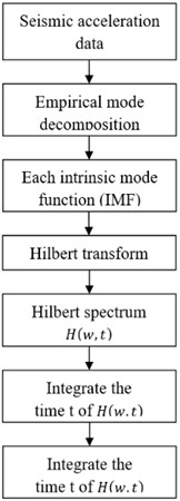
The Hilbert-Huang Transform (HHT) is an advanced tool for analyzing nonlinear and non-stationary time series signals, capable of effectively capturing the spectral characteristics of slopes under seismic excitation. The analysis of seismic responses of living stumps within slopes using the HHT method primarily consists of two parts: Empirical Mode Decomposition (EMD) and the Hilbert transform. The EMD method assumes that seismic waves are composed of a set of intrinsic mode functions (IMFs). Each IMF component must satisfy two conditions: (1) in the time series, the number of extrema and zero-crossings must either be equal or differ by at most one; and (2) the mean of the upper and lower envelopes defined by the local maxima and minima must be zero. Subsequently, the Hilbert transform is applied to the decomposed IMFs to obtain the instantaneous spectral characteristics of each IMF component. By integrating the instantaneous spectra of all IMF components, the Hilbert energy spectrum (HHT spectrum) can be derived. The Hilbert transform of IMF $c\left(t\right)$ is expressed as follows:

where, $PV$ denotes the Cauchy principal value. The analytic signal $z\left(t\right)$ is constructed as follows:

where, $a\left(t\right)$ represents the amplitude function, and $\mathrm{\Phi }\left(t\right)$ denotes the phase function:

Based on the aforementioned formulas, the Hilbert transform is applied to the IMF components to obtain the energy distribution characteristics of seismic waves in the time-frequency domain. The formula for the Hilbert spectrum is as follows:

Finally, integrating $H(\omega ,t)$ over time yields the marginal spectrum:

The application process of the time-frequency analysis method based on HHT in the seismic response of living stumps within slopes is shown in Fig. 14.

4.1. HHT energy spectrum analysis

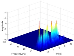
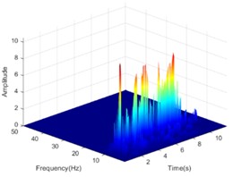
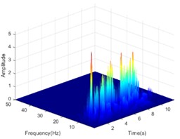
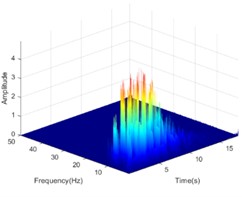
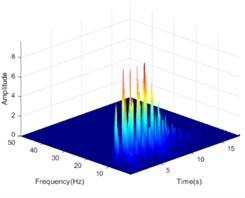
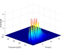
The Hilbert-Huang transform (HHT) is a reliable tool to clarify the propagation characteristics of seismic energy in the time-frequency domain. In view of the length of the article, only the HHT energy spectrum on both sides of the living stumps is given when the excitation intensity is 0.4 g K-XZ and DR-XZ (see Fig. 15 and Fig. 16). It can be seen from Fig. 15 and Fig. 16 that when the seismic wave propagates inside the slope, the HHT energy spectrum has multiple peaks. These peaks are dispersed on the time axis, and the main distribution ranges in the time domain and frequency domain are 0-12 s and 0-15 Hz. It is noteworthy that the HHT energy spectrum peaks (PSHEA) appear in the range of 5-15 Hz, indicating that seismic waves carry a significant amount of seismic Hilbert energy within this frequency range, which has a substantial impact on the dynamic response of the living stumps slope. Fig. 15 compares the HHT energy spectra of the inner monitoring points (#9-#11) with the outer monitoring points (#6-#8) of the living stumps. The results show that the HHT energy spectrum gradually decreases during the propagation of seismic waves, resulting in a lower PSHEA at the outer monitoring point (#6-#8) than the inner monitoring point (#9-#11).

Fig. 14Flow chart of HHT analysis method

This difference causes different dynamic responses on both sides of the living stumps, and further reveals the dynamic response law of the slope supported by the living stumps. Additionally, as the seismic waves propagate through the living stumps, the high-frequency and low-frequency components of the internal and external monitoring points of the living stumps are attenuated, but the attenuation degree of the low-frequency component is much larger than that of the high-frequency component. This difference may be due to the fact that the living stumps not only filters the frequency component of the seismic wave, but also combines the surrounding rock and soil to filter the low frequency component and amplify the high frequency component. Meanwhile, as shown in Fig. 15, during the seismic propagation process from the slope bottom to the slope top, the living stumps slope exhibits significant characteristics of amplifying high-frequency components and filtering low-frequency components. In this process, the PSHEA gradually increased with the increase of slope height. The change of PSHEA at the monitoring point outside the living stumps is shown in Fig. 17. As seen in Fig. 17(a), the PSHEA is positively correlated with elevation and excitation intensity. At the foot of the slope, with the increase of excitation intensity, the growth rate of PSHEA is slower; at the top of the slope, with the increase of excitation intensity, the growth rate of PSHEA is faster. Specifically, when the excitation intensity increases from 0.1 g to 0.6 g, the PSHEA at the foot of the slope increases from 1.421 to 7.462, and the PSHEA at the top of the slope increases from 2.768 to 15.032. This indicates that the variation trend of the HHT energy spectrum with excitation intensity is affected by elevation. Specifically, as the elevation increases, the increase of PSHEA with the rise in excitation intensity becomes more pronounced.

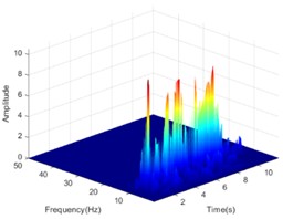
Under the action of DR-XZ with an excitation intensity of 0.4 g, the HHT energy spectrum and PSHEA variation patterns of the measurement points on both sides of the living stumps are shown in Fig. 16 and Fig. 17(b), respectively. As shown in the figure, it can be seen that under the action of DR-XZ, the HHT energy spectrum variation patterns at the measurement points on both sides of the living stumps are similar to those under the K-XZ condition. When seismic waves propagated through the living stumps, differences in the HHT energy spectrum were observed at the measurement points on both sides of the living stumps. Whether it is inside or outside of the living stumps, the seismic Hilbert energy and PSHEA increase with the increase of elevation, and are positively correlated with the excitation intensity. Comparing Fig. 15 and Fig. 16, as well as Fig. 17(a) and Fig. 17(b), it can be seen that under the action of different types of seismic waves, the HHT energy spectrum and PSHEA of the monitoring points on both sides of the living stumps are different in value, but the change trend is similar. This shows that the type of seismic wave mainly affects the values of the seismic Hilbert energy spectrum and PSHEA, but has little impact on their variation trends.

Fig. 15The HHT energy spectrum on both sides of the living stump under the action of K-XZ with excitation intensity of 0.4 g

a) Outside #6

b) Outside #7

c) Outside #8

d) Inside #9

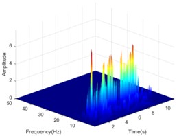
e) Inside #10

f) Inside #11

Fig. 16The HHT energy spectrum on both sides of the living stump under the action of DR-XZ with excitation intensity of 0.4 g

a) Outside #6

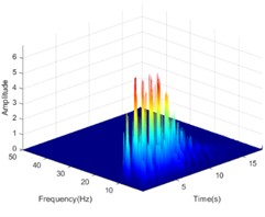
b) Outside #7

c) Outside #8

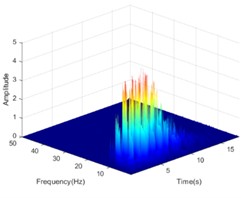
d) Inside #9

e) Inside #10

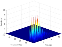
f) Inside #11

Fig. 17The PSHEA on the Outside of the living stumps under different excitation intensities and different seismic waves

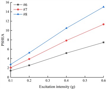
a) KB-XZ

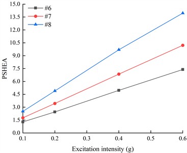
b) DR-XZ

4.2. Marginal spectrum analysis

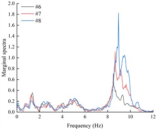
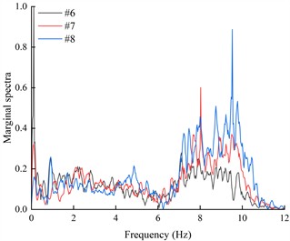
The marginal spectra of each acceleration measurement point were obtained by integrating the HHT energy spectra over time, in order to investigate the variation of seismic Hilbert energy on both sides of the living stumps within the slope. Due to space limitations, this paper presents only the marginal spectra of acceleration monitoring points #6, #7, and #8 located on the outer side of the living stumps under K-XZ and DR-XZ excitations with different intensities (see Fig. 18 and Fig. 19).

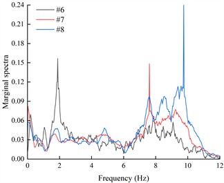
It can be seen from Fig. 18 that under the action of different excitation intensity K-XZ, the marginal spectra of monitoring points #6, #7, and #8 exhibit three peaks: the first peak occurs within the frequency range of 1-3 Hz, the second within 4-6 Hz, and the final one within 7-11 Hz. Regardless of the frequency range, the marginal spectral curves of the three monitoring points show similar variation trends. In the lower frequency ranges (1-3 Hz and 4-6 Hz), the peak values of the marginal spectra (PMSA) for #6, #7, and #8 are comparable and increase gradually with increasing excitation intensity. In the higher frequency range (7-11 Hz), although the PMSA of all three points is positively correlated with excitation intensity, notable differences exist among them, and these differences increase progressively with increasing excitation intensity. As observed in Fig. 18, under the action of K-XZ at 0.1g, the PMSA at monitoring points #7 and #8 appear at the same frequency. However, under other excitation intensities (0.2 g, 0.4 g, and 0.6 g), there is a certain degree of lag, meaning that the PMSA don’t occur at the same frequency. This may be attributed to the inherent spectral characteristics of seismic waves and the filtering effect of living stumps, which attenuate low-frequency components and amplify high-frequency components. The effect becomes more pronounced with increasing excitation intensity and elevation, thereby leading to a lag in the marginal spectrum peaks under other excitation intensities.

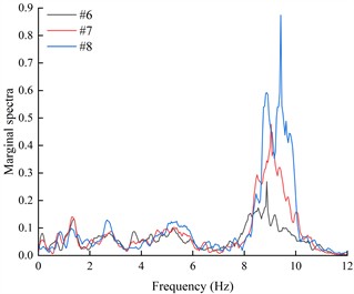
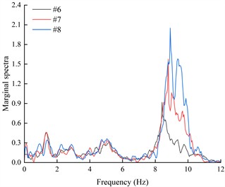
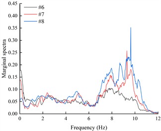
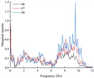
Fig. 19 shows the variation of the marginal spectral curves of monitoring points #6, #7, and #8 under the action of DR-XZ with different excitation intensities. As shown in Fig. 19, under the action of DR-XZ, the marginal spectra of #7 and #8 exhibit three peaks within the same frequency ranges as observed under K-XZ excitation: 1-3 Hz, 4-6 Hz, and 7-11 Hz. Notably, within the 1-3 Hz and 7-11 Hz frequency ranges, the marginal spectrum of #6 is similar to that under K-XZ excitation, showing clear peaks, whereas no distinct peak is observed within the 4-6 Hz frequency range. In summary, within the 1-3 Hz and 7-11 Hz frequency ranges, the marginal spectral curves of #6, #7, and #8 under DR-XZ excitation show similar trends to those under K-XZ excitation, although numerical differences are present. Within the 4-6 Hz frequency range, the marginal spectra of #7 and #8 first increase and then decrease with frequency, while that of #6 exhibits a decreasing trend with increasing frequency. This phenomenon may be attributed to the location of #6 at the slope toe, where the surrounding soil is relatively stable. Additionally, the living stumps work together with the soil near the toe to filter out low-frequency components of seismic waves, resulting in a continuous reduction in energy within the 4-6 Hz frequency range. Consequently, the seismic Hilbert energy at the slope toe is lower, leading to reduced dynamic response compared to the mid-slope and crest. By comparing Fig. 18 and Fig. 19, it can be concluded that the type of seismic wave primarily affects the magnitude of the marginal spectra and the trend of the marginal spectrum at the slope toe (#6) within the low-frequency range, but has minimal influence on the variation trends of the marginal spectra within the high-frequency range for monitoring points #6, #7, and #8.

Fig. 18The marginal spectra of monitoring points on the outside of living stumps under different excitation intensities of K-XZ

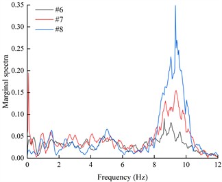
a) 0.1 g

b) 0.2 g

c) 0.4 g

d) 0.6 g

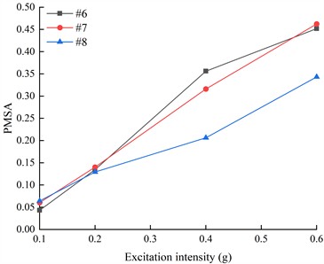
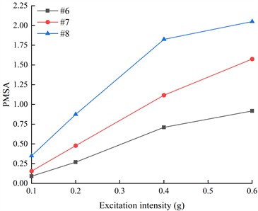
Considering that there are only two peaks in the marginal spectrum of # 6 under the action of DR-XZ, the PMSA of the measuring points outside the living stumps in the frequency range of 1-3 Hz and 7-11 Hz under the action of K-XZ and DR-XZ with different excitation intensities were selected for comparison, as shown in Fig. 20 and Fig. 21. Under the action of K-XZ with different excitation intensities, when the frequency is in the range of 7-11 Hz, the PMSA of #6, #7 and #8 is significantly positively correlated with the excitation intensity. Moreover, the PMSA of #8 is significantly higher than that of #6, and this difference increases progressively with increasing excitation intensity. This indicates that as elevation and excitation intensity increase, seismic Hilbert energy accumulates during upward propagation, with high-frequency (7-11 Hz) components of seismic waves being notably amplified. Within the frequency range of 1-3 Hz, the PMSA of monitoring points #6, #7, and #8 gradually increases with excitation intensity; however, at this point, the PMSA of #8 is significantly lower than that of #6 and #7. Combined with previous analysis of high-frequency (7-11 Hz) PMSA, it is evident that as elevation and excitation intensity increase, the slope supported by living stumps filters out low-frequency components while amplifying high-frequency components, leading to a gradual decrease in low-frequency (1-3 Hz) seismic Hilbert energy and its transfer to high-frequency (7-11 Hz) components. Consequently, the low-frequency seismic Hilbert energy at the crest is minimized, while the high-frequency seismic Hilbert energy is maximized. This phenomenon strongly corroborates the previously mentioned characteristic of slopes supported by living stumps to filter low-frequency components and amplify high-frequency components of seismic waves [40].

Fig. 19The marginal spectra of monitoring points on the outside of living stumps under different excitation intensities of DR-XZ

a) 0.1 g

b) 0.2 g

c) 0.4 g

d) 0.6 g

As shown in Fig. 20 and Fig. 21, the PMSA monitoring points exhibit overlapping in the low-frequency range (1-3 Hz), but show significant separation in the high-frequency range (7-11 Hz). In the low-frequency range, the overlap of PMSA monitoring points may be attributed to the overall stiffness and mass distribution of the slope system dominating its dynamic behavior, indicating that seismic effects are relatively uniform across the slope, leading to a more consistent dynamic response. Additionally, low-frequency vibrations are more susceptible to viscous damping effects within the soil medium, which can effectively dissipate seismic energy, thereby causing the PMSA monitoring points to overlap in the low-frequency range. In the high-frequency range (7-11 Hz), the significant separation of PMSA monitoring points may result from high-frequency vibrations being more likely to induce localized stress concentrations within and on the surface of the slope, while the energy distribution of seismic waves changes significantly with frequency. Within this frequency range, differences in seismic wave propagation paths, velocities, and attenuation characteristics become more pronounced, leading to variations in slope response patterns, as evidenced by the clear separation of PMSA monitoring points, and under high-frequency seismic input, the dynamic response of living stumps and the surrounding soil exhibits higher complexity. Specifically, the combined effects of refraction and reflection of seismic waves by the living stumps, along with their filtering of low-frequency components and amplification of high-frequency components, together with viscous damping in the soil, intensify the non-uniformity of the slope response, resulting in the separation of PMSA values.

A comparison was conducted of PMSA at frequencies within the 1-3 Hz and 7-11 Hz ranges from monitoring points on the outer side of living stumps under DR-XZ and K-XZ excitations with varying intensities. The results indicate that, regardless of whether in the low-frequency (1-3 Hz) or high-frequency (7-11 Hz) range, during upward propagation of seismic waves, the variation trends of PMSA with excitation intensity are similar under both types of seismic waves, although differences exist in their magnitudes. Notably, within the low-frequency range, the variation trend of PMSA with elevation is opposite to that observed in the high-frequency range. These findings suggest that the type of seismic wave primarily affects the magnitude of PMSA, with minimal influence on the ability of slopes supported by living stumps to filter out low-frequency components and amplify high-frequency components.

Fig. 20The PMSA of monitoring points on the outside of living stumps in the frequency range of 1-3 Hz

a) K-XZ

b) DR-XZ

Fig. 21The PMSA of monitoring points on the outside of living stumps in the frequency range of 7-11 Hz

a) K-XZ

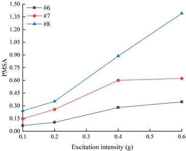
b) DR-XZ

The marginal spectrum characterizes the contribution of any frequency value in the signal to the total seismic Hilbert energy [41]. Therefore, the marginal spectral curves in Fig. 18 and Fig. 19 were integrated, and the area below the marginal spectral curve represents the total seismic Hilbert energy in the whole frequency range. In the living stumps slope, the total seismic Hilbert energy of the monitoring points located on the inside of the living stumps (#9, #10, and #11) and the outside (#6, #7, and #8) is shown in Fig. 22.

Fig. 22(a) shows the total seismic Hilbert energy of the monitoring points on both sides of the living stumps under the action of different excitation intensities K-XZ. As shown in the figure, regardless of the variation in excitation intensity, the total seismic Hilbert energy is highest at the top of the slope (points #8 and #11), followed by the middle of the slope (points #7 and #10), and lowest at the bottom of the slope (points #6 and #9) in the living stumps slope. Meanwhile, with the increase of excitation intensity, the total seismic Hilbert energy of the monitoring points on both sides of the living stumps gradually increases, and reaches the maximum value when the excitation intensity is 0.6 g. For example, when the excitation intensity increases from 0.1 g to 0.6 g, the total seismic Hilbert energy at monitoring point #8 increases from 0.609 to 3.531. This strongly verifies the previously stated point of view that with the increase of elevation and excitation intensity, the seismic Hilbert energy tends to accumulate upward and reach the maximum at the top of the slope. Additionally, the total seismic Hilbert energy on the outside of the living stumps comes from the energy carried by seismic waves propagating through the living stumps, as well as the energy accumulated during the upward propagation of the seismic waves. Therefore, exploring the distribution characteristics of the total seismic Hilbert energy on both sides of the living stumps is of great significance for revealing the dynamic response mechanism of slopes supported by living stumps. As shown in Fig. 22(a), it can be seen that the total seismic Hilbert energy of the monitoring points outside the living stumps is always smaller than that inside the living stumps, whether it is the top of the slope (#8 and #11), the middle of the slope (#7 and #10), or the foot of the slope (#6 and #9). For example, when the K-XZ with an excitation intensity of 0.6g propagates from #10 to #7, the seismic Hilbert energy decreases from 2.757 to 2.576. In the studies by Fan [42, 43], it was found that for slopes without any support measures, the total seismic Hilbert energy in the horizontal direction gradually increased from the interior of the slope towards the slope surface under seismic loading. However, in this study, for slopes supported by living stumps, the total seismic Hilbert energy inside the living stumps was consistently higher than that on the outer side under seismic loading. This indicates that during the propagation of seismic waves, due to the combined effects of reflection and refraction at the surface of living stumps, as well as energy absorption, living stumps exhibit a significant attenuation characteristic for the total seismic Hilbert energy [44-47]. Moreover, as elevation and excitation intensity increase, the attenuation degree of the total seismic Hilbert energy by the living stumps gradually increases. For example, under the action of 0.4g K-XZ, the energy values of total seismic Hilbert energy attenuation from the foot to the top of the slope were 0.061, 0.088, and 0.110, respectively.

Fig. 22The total Hilbert energy of the earthquake at the monitoring points on the left and outsides of the living stumps under different excitation intensities and different seismic waves

a) K-XZ

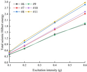
b) DR-XZ

Fig. 22(b) is the variation law of the action of DR-XZ with different excitation intensities. As shown in the figure, with the increase of elevation and excitation intensity, the seismic Hilbert energy on both sides of the living stumps increases gradually, the seismic Hilbert energy on both sides of the living stumps gradually increased, and the seismic Hilbert energy of the inner monitoring points was always greater than that of the outer monitoring points. Under the action of DR-XZ, the living stumps exhibited an attenuation effect on the total seismic Hilbert energy, and the attenuation degree is also positively correlated with the elevation and the excitation intensity. Specifically, the higher the elevation and the greater the excitation intensity, the greater the attenuation of the total seismic Hilbert energy caused by the living stumps. For example, when the excitation intensity was 0.2 g, the values of seismic Hilbert energy attenuation from slope toe to slope top were 0.021, 0.025 and 0.084, respectively. This shows that the attenuation degree of seismic wave energy by living stumps is mainly affected by elevation and excitation intensity, with little correlation to the type of seismic wave.

5. Discussion

In the large-scale shaking table test of slopes supported by living stumps, the difference in acceleration time histories inside and outside the living stumps indicates a significant disparity in the dynamic response on both sides. To further investigate the causes of this dynamic response difference, the study utilized HHT energy spectra and marginal spectra to conduct an in-depth analysis from the perspectives of seismic Hilbert energy distribution and time-frequency characteristics. During the propagation of seismic waves within the slope supported by living stumps, the superposition of incident and refracted waves at the stump surface, along with energy absorption, leads to an attenuation effect on the total seismic Hilbert energy. As a result, the seismic Hilbert energy outside the living stumps is lower than that inside. This difference in seismic Hilbert energy on both sides of the living stumps results in distinct dynamic responses inside and outside the stumps. When seismic waves pass through the living stumps, both low-frequency (1-3 Hz) and high-frequency (7-11 Hz) components are attenuated; however, the attenuation of low-frequency components is significantly greater than that of the high-frequency components. This is because, in addition to the attenuation effect, living stumps also exhibit characteristics of filtering out low-frequency components and amplifying high-frequency components, leading to a transfer of seismic Hilbert energy from the low-frequency range (1-3 Hz) to the high-frequency range (7-11 Hz), further concentrating the seismic Hilbert energy in the high-frequency components of the seismic waves. Furthermore, the acceleration difference between both sides of the living stumps is greatest at the slope crest, followed by the mid-slope, and smallest at the slope toe. This indicates that the absolute value of the acceleration difference increases with elevation and excitation intensity, a trend consistent with the increasing attenuation of total seismic Hilbert energy by the living stumps as elevation and excitation intensity increase. The similarity in these variation patterns further demonstrates their close relationship, indicating that the acceleration response of slopes supported by living stumps serves as an external manifestation of the total seismic Hilbert energy.

In the study by Niu [44], rubber rods were embedded in a clay slope to simulate the root system of Sophora viciifolia, and shaking table tests were conducted. It was found that the total energy of vegetated slopes was lower than that of bare slopes. Although the rubber rods could reasonably simulate the mechanical properties of Sophora viciifolia roots, the actual root system consists of vertical primary roots, lateral roots, and fine roots. The experiment simulated only the vertical primary roots and did not account for the spatial distribution of lateral roots or their synergistic reinforcement effects, which may have led to an over-idealization of the root system’s resistance to sliding. However, in this study, a root system model was constructed using 3D printing technology, fully incorporating the structural characteristics of lateral roots. This approach resulted in a model that more closely resembled real root systems in both geometric shape and mechanical behavior, effectively addressing issues of poor geometric repeatability and mechanical distortion present in traditional models. In the study by Liang [14], a tree root model was constructed using 3D printing technology and centrifuge tests were conducted. It was found that root systems can significantly reduce seismic-induced crest settlement in slopes. In his study, the analysis was primarily based on experimentally obtained seismic response data of slopes, with the methodology limited to traditional mechanical and displacement-based perspectives, focusing on low-frequency dynamic responses. However, this study employed the HHT analysis method to process the collected seismic response data of slopes, enabling the quantification of time-frequency characteristics and energy distribution changes within nonlinear systems. This approach reveals the high-frequency dynamic response features and detailed response mechanisms of living stump-supported slopes under seismic loading, providing a new analytical framework for evaluating the reinforcing effects of root systems on slopes under earthquake conditions.

In this study, a living stump model was constructed using 3D printing technology, and the dynamic characteristics of the slope supported by living stumps under seismic loading were analyzed based on time-frequency features and energy variation characteristics using the HHT method. The geometric morphology of plant roots has a significant influence on the stability of slopes under seismic loading. Therefore, future studies will focus on the development of more sophisticated root system models for living stumps to enhance the representation of their root structures. Additionally, three-dimensional numerical models under various loading conditions will be developed using finite element software, and a comprehensive analysis will be conducted by integrating computational results with experimental data to further investigate the supporting mechanisms and effectiveness of living stumps on slope stability under seismic conditions.

6. Conclusions

This study designed and conducted a large-scale shaking table test of slopes supported by living stumps with a geometric similarity ratio of 1:7. Horizontal acceleration responses on both sides of the living stumps under different excitation intensities (K-XZ and DR-XZ) were obtained. HHT energy spectra and marginal spectra from monitoring points on either side of the living stumps were analyzed using Hilbert-Huang Transform to investigate their time-frequency and energy variation characteristics, thereby further analyzing the dynamic response of slopes supported by living stumps. The main conclusions are as follows:

1) Inside the slope supported by living stumps, the peak horizontal acceleration is positively correlated with excitation intensity and elevation. Additionally, there is a difference in horizontal acceleration between both sides of the living stumps, and the absolute value of this difference increases with elevation and excitation intensity, particularly noticeable in peak horizontal acceleration. The type of seismic wave mainly affects the numerical values of horizontal acceleration but has little influence on its variation patterns.

2) Under different seismic waves, the peak value of HHT energy spectrum (PSHEA) is positively correlated with excitation intensity and elevation. Furthermore, as elevation increases, the increase in PSHEA with increasing excitation intensity becomes more pronounced. The peak value of the marginal spectrum (PMSA) is positively correlated with excitation intensity; however, at low frequencies (1-3 Hz), PMSA is negatively correlated with elevation, while at high frequencies (7-11 Hz), it is positively correlated with elevation.

3) Regardless of the type of seismic wave, as elevation and excitation intensity increase, the total seismic Hilbert energy accumulates along the elevation and reaches its maximum at the slope crest. Meanwhile, the living stumps and soil-rock mass within the slope effectively filter out low-frequency components (1-3 Hz) and amplify high-frequency components (7-11 Hz). The total seismic Hilbert energy in the low-frequency range decreases with elevation and shifts to the high-frequency range, significantly increasing the total seismic Hilbert energy in the high-frequency components.

4) Seismic waves carry a significant amount of total seismic Hilbert energy within the frequency range of 5-15 Hz. Due to the superposition of incident and reflected waves near the living stumps and the absorption of total seismic Hilbert energy by the living stumps, the PSHEA, PMSA, and total seismic Hilbert energy outside the living stumps are consistently lower than inside, resulting in different dynamic responses on both sides. Living stumps exhibit an attenuation effect on seismic Hilbert energy, which increases with excitation intensity and elevation.