A vision-based deep learning approach for non-contact vibration measurement using (2+1)D CNN and optical flow

1.1. Background

The nature of the maintenance approach is moving from corrective to preventive and, in the future, predictive. Predictive maintenance detects trends and anticipates the problems before they arise [1]. This approach only performs equipment maintenance when necessary, thus saving maintenance costs and maximizing operation. Predictive maintenance uses condition-based monitoring, machine learning, and analytics techniques to predict upcoming machine or asset failures. Condition-based monitoring (CBM) requires high-performance sensors, including accelerometers, pressure sensors, MEMS microphones, etc. [2], [3]. However, the most functional sensors are the accelerometers for detecting vibration, an important starting parameter for predictive maintenance [4]. In the context of vibration detection, conventional piezoelectric accelerometers, often regarded as the gold standard, are less suitable for wireless predictive maintenance systems due to limitations in size, lack of integrated features, and high-power consumption [5]. Additionally, the installation of these sensors may be difficult and expensive [6-8]. To overcome these limitations, non-contact sensing techniques have been developed and can be broadly categorized into laser-based, vision-based, and deep learning-driven approaches. A widely used laser-based method is the laser Doppler vibrometer (LDV), which offers high precision but suffers from drawbacks related to cost, bulkiness, and limited accessibility [9]. Moreover, since a laser is a concentrated beam of energy, it can raise the surface temperature of the object under measurement, making it potentially invasive and capable of altering the object's natural vibration frequency [10, 11]. As an alternative, vision-based sensing methods have gained attention due to their low cost, ease of deployment, and non-invasiveness. These include techniques such as digital image correlation (DIC), optical flow analysis, and deep learning-based models that infer structural vibration responses directly from video data. Among these, vision-based neural networks are emerging as a promising solution for modal analysis and multi-parameter vibration estimation.

1.2. Existing methods of non-contact vibration measurement

1.3. Paper contribution

Despite the potential of 3D CNNs for vibration measurement, no research has explored their application or developed models based on this framework in this domain. Existing studies have primarily relied on CNN-LSTM models, which focus predominantly on shape frequency prediction and lack a comprehensive analysis of other vibration metrics. To address this gap, this study proposes leveraging recent advancements in 3D CNNs, specifically the factorization of kernels into the (2+1)D CNN architecture, to enhance vibration measurement analysis.

This paper presents a novel non-contact vibration measurement framework that uniquely combines a (2+1)D CNN with optical flow preprocessing to simultaneously predict acceleration, velocity, displacement, and frequency from video inputs. Unlike prior vision-based methods that address only one or two metrics, our approach delivers a holistic solution by regressing all four key vibration parameters, marking a significant departure from conventional techniques. The integration of optical flow addresses critical data desynchronization issues, enabling precise temporal alignment between video frames and vibration signals. The model also aims to adapt in varying light levels and camera-object distances without the calibration required by pure image processing methods like DIC or optical flow, ensuring robustness across diverse environments.

2.1. Four-output regression (2+1) dimension CNN

Predicting acceleration, velocity, displacement, and frequency from sequences of images requires effective modeling of temporal information. Traditional two-dimensional (2D) CNNs are limited in this regard, as they process frames independently and cannot capture temporal dynamics. Three-dimensional (3D) CNNs address this limitation by extracting spatiotemporal features across consecutive frames; however, they introduce substantial computational overhead. To balance temporal modeling capability with computational efficiency, a 3D CNN can be factorized into a (2+1)D CNN, which separates spatial and temporal convolutions while preserving temporal awareness [33]. This architecture supports the use of 3D CNNs over alternatives such as CNN–LSTM models, which, although previously applied to modal frequency prediction, were restricted to shape frequency and did not address other key vibration parameters.

Fig. 1Overall Structure of the proposed model and its residual layer content

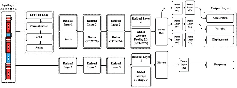
a) Overall Structure of (2+1) D CNN-based model

b) Contents of the residual layer

Fig. 1 illustrates the architecture of the proposed four-output regression model based on (2+1)D CNN. The model comprises several distinct processing stages designed to handle spatiotemporal vibration data analysis. The input layer accepts three-dimensional data, where the first two dimensions represent spatial frame information (height × width) and the third dimension corresponds to temporal information (number of sequential frames). This input undergoes parallel processing through two distinct convolutional operations: a 2D spatial convolution analyzing frame content and a 1D temporal convolution examining pixel evolution across frames. Following the input layer, the (2+1)D CNN layer performs initial feature extraction, subsequently normalized and down-sampled through dimensionality reduction.

The architecture then incorporates multiple residual blocks, each performing progressive downscaling. These residual connections serve two critical functions: mitigating model degradation during deep network training and enhancing discriminative feature extraction. The hierarchical downscaling process enables the model to selectively focus on relevant frame regions while suppressing extraneous information, including background noise and lighting artifacts. The final stages employ 3D pooling operations followed by feature vector flattening, transforming the spatiotemporal data into a compact representation. This distilled feature set feeds into four specialized hidden layers, each optimized for predicting one of the four target vibration metrics.

The (2+1)D CNN architecture was selected for its balance of computational efficiency and temporal modeling capability.

2.2. Equipment and experiment setup

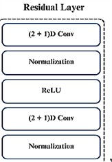
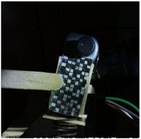
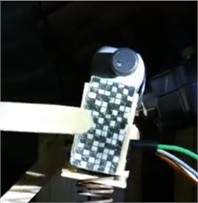
The experiment setup is shown in Figs. 2 and 3, which consists of a vibration motor, a vibration meter, an accelerometer sensor, a Raspberry Pi 5 with a camera, an illumination source, and a computer. At the core of this setup is a vibration motor, which generates controlled oscillatory motion. The vibrations affect a cube to which the motor is attached. To quantify these vibrations, a vibration meter and an accelerometer (MPU6050) are placed directly in contact with the cube to get the most accurate reading of acceleration, velocity, and displacements. The accelerometer continuously records acceleration data over time, which is later processed to compute vibration frequency.

Fig. 2Experiment setup diagram

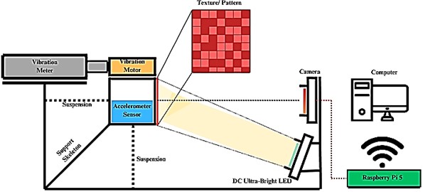
Fig. 3Actual setup. Image credit: Harold Harrison, UMS Faculty of Engineering Laboratory, 2024

This setup employs two ESP-32 microcontrollers to ensure reliable operation. The first microcontroller regulates the vibration motor to control the magnitude of vibration velocities, while the second records acceleration data from the accelerometer. Using separate ESP-32 units prevents interference between motor control and sensor sampling, which could otherwise compromise measurement accuracy. Although parallel programming on a single ESP-32could theoretically achieve similar functionality, preliminary testing showed that multi-threading leads to excessive heat generation causing system instability. Furthermore, this study found that combining high-frequency sensor sampling with motor control on a single microcontroller resulted in frequent system crashes.

An essential component of the experimental setup involves applying a textured pattern to the surface of the cube to enhance motion tracking accuracy by improving shift and displacement detection. A Raspberry Pi 5 camera, positioned at a distance from 10 to 50 cm perpendicular to the cube, captures video footage at high frame rates. The video stream is transmitted in real time to a dedicated processing computer via a Flask-based server system, enabling immediate preprocessing and model training.

To maintain image clarity under high shutter speeds, an external DC-powered ultra-bright LED light source provides consistent illumination. Data collection is conducted under two distinct environmental conditions: (1) a semi-controlled laboratory setting with variable ambient lighting (including natural light from windows and artificial ceiling lighting) and (2) an open space to simulate real-world scenarios. This approach ensures dataset diversity in illumination levels, further augmented by varying LED light levels. Representative video frames illustrating different lux configurations are provided in Fig. 4, demonstrating the range of illumination conditions incorporated into the dataset.

Fig. 4Single frame at a) 50 lux, b) 300 lux. Image credit: Harold Harrison, UMS Faculty of Engineering Laboratory, 2024

a)

b)

Visualizing vibrational motion requires the analysis of four fundamental kinematic parameters: displacement, velocity, acceleration, and frequency. Displacement is determined by tracking the positional coordinates of a reference point over time, with temporal resolution provided by synchronized timestamps. Velocity and acceleration are subsequently derived through first- and second-order temporal differentiation of the displacement data, respectively. Frequency characterization, representing the system’s predominant oscillation rate, is typically obtained via spectral analysis of periodic motion. This is most commonly achieved through computational methods such as the Fast Fourier Transform (FFT) or related signal processing techniques that decompose the time-domain signal into its constituent frequency components.

Accurate frequency measurement requires adherence to the Nyquist sampling theorem, which specifies that the sampling rate must be at least twice the highest frequency component of interest. Given that typical machinery operates below 60 Hz [34], a minimum sampling rate of 120 Hz is required for reliable measurement. In the context of optical measurement, the sampling rate corresponds to the camera’s frame rate, necessitating a capture capability of at least 120 frames per second (fps). This study employs a Raspberry Pi 5 equipped with a high-speed camera module capable of exceeding 120 fps, thereby satisfying the Nyquist criterion for the target frequency range. Theoretically, this configuration enables accurate vibration measurement across the 1-60 Hz spectrum, encompassing the operational frequencies of most mechanical systems.

2.3. Acquisition of videos, vibration data and preprocessing

The vibration measurement and video recording methodology are illustrated in Fig. 5. A calibrated vibration meter is employed to quantify vibrations induced by the motor, with the sensor positioned atop the cube in direct structural contact. This configuration ensures optimal sensor coupling while accounting for the sensor’s mass contribution to the overall system load, thereby improving measurement consistency. The vibration meter provides direct readings of acceleration, velocity, displacement, and frequency range.

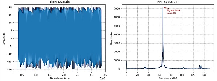
For precise frequency determination, a triaxial accelerometer (MPU6050) with a 300 Hz sampling capability supplements the vibration meter measurements. During synchronous video recording, the acquired acceleration data is logged for subsequent spectral analysis via Fast Fourier Transform (FFT) (Fig. 6). To validate measurement integrity, FFT-derived frequencies are cross-verified against the vibration meter's indicated range; any discrepancies result in data exclusion from further analysis.

Fig. 5Data collection flow-chart

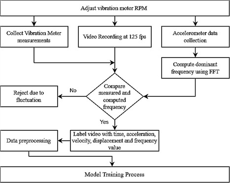
Fig. 6Time-domain signal and corresponding FFT spectrum of MPU6050 acceleration data

As the primary goal is to establish proof-of-concept feasibility, the MPU6050’s programmable ranges (±2 g to ±16 g) and 16-bit resolution provide adequate performance to capture general vibration trends in controlled settings, offering sufficient data to demonstrate correlations between video inputs and vibration outputs during the initial development phase. Furthermore, its use establishes a scalable baseline, paving the way for future enhancements by identifying model strengths and weaknesses that can be addressed with more precise sensors in subsequent work. For future research, it is recommended to incorporate high-precision equipment, such as industrial-grade accelerometers, to improve accuracy and robustness as the model progresses toward real-world deployment.

The Raspberry Pi captures video footage at a frame rate of 125 fps. Certain settings were adjusted to enable high-speed frame capturing. One key modification was reducing the resolution to 640×640 pixels to minimize the GPU workload. The shutter speed was set to 1/300 seconds, and the Libav codec was selected, as other codecs impose a maximum recording frame rate of less than 120 fps. Additionally, the default denoise feature of the libcamera-vid library, which is commonly used with the Pi camera, was disabled to conserve GPU resources during video recording. A frame processing function was developed to process all recorded video data efficiently. This function accepts several parameters, including the frame resolution, the total number of frames, and the spacing between extracted frames. During development, the resolution and frame count were carefully tuned and optimized to enhance performance. The frame processing function begins by scanning video files that adhere to a specific naming convention: a{A}_v{V}_d{D}_f{F}.mp4', where 'A' represents acceleration, 'V' represents velocity, 'D' represents displacement, and 'F' represents frequency measurements.

To address the limited size of the dataset, particularly concerning the frequency spectrum, data augmentation was performed by rendering the same collected videos at varying playback speeds (either faster or slower). This approach expanded the frequency range of the dataset to span 5 to 80 Hz. The resulting videos are all rendered at a constant 300 fps for the sole purpose of testing if the frame speed does affect the range of frequency that the model can predict. Additionally, to enhance diversity in illumination conditions, videos were captured using different shutter speeds, thereby increasing variability in lighting levels across the dataset.

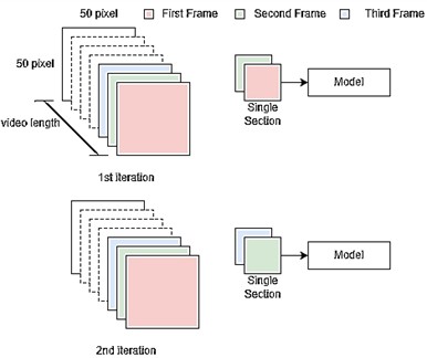
Each video filename encapsulates all relevant vibration measurement labels, ensuring clarity in dataset organization. Once identified, frames are extracted at a specified depth (i.e., the number of frames input into the model). The function also supports multi-section frame extraction, allowing multiple segments of frames to be retrieved from a single video, maximizing the utilization of the dataset. For example, in a 4-second video recorded at 125 frames per second (fps), a total of 500 frames is available. The multi-sectioning method enhances dataset efficiency by enabling multi-sampling of frames, reducing frame wastage. Fig. 7 illustrates this multi-sectioning approach in detail.

Fig. 7Multi-section frame sampling of a depth of two in a single video

Once the frames and labels are organized, the dataset is split into a training set (80 %) and a validation set (20 %). Within the validation dataset, a sub-segment is designated as the testing dataset, which is used to evaluate and showcase the model’s performance. Initial data collection consists of 100 4-second videos. After going through the optical flow validation algorithm, around 2000 videos were created, consisting of five frames in each video while maintaining the same time interval between each frame.

2.4. Performance metric

For model evaluation, the Mean Absolute Percentage Error (MAPE) metric is employed alongside the Root Mean Square Error (RMSE) and the Coefficient of Determination ($R^2$). The rationale for choosing MAPE is that it enables the detection of individual measurements that may underperform or outperform expectations, providing a more interpretable measure of error in percentage terms. Since the dataset contains measurements at varying scales, MAPE offers a more standardized error assessment [35], making it a suitable loss function for model training. RMSE is included to measure the average magnitude of the errors in the predicted values, giving higher weight to larger errors, which is useful for understanding the spread of prediction errors. $R^2$ is utilized to assess the proportion of variance in the dependent variable that is predictable from the independent variables, providing insight into the goodness of fit of the model.

To be considered reliable, the MAPE must be below 30 %, as values beyond this threshold suggest that the model is engaging in random guessing rather than effectively generalizing the dataset. The performance is considered acceptable if MAPE falls under 30 %, good within the range of 10 % to 20 %, and excellent performance if it falls below 10 %. For RMSE, a lower value indicates better performance, with the threshold for acceptability depending on the scale of the data. An $R^2$ value closer to 1 indicates a better fit, with values above 0.7 generally considered acceptable, above 0.9 indicating good performance, and values near 1 reflecting excellent performance.

3.1. Initial model

The input to the initial model is the consecutive frames without any pre-processing. Initially, the training starts with two depth frames, which are gradually increased to 60 depth frames to determine the optimal performance. Several input resolutions are also tested to identify the most effective configuration. The optimization process involves tuning the (2+1)D CNN hyperparameters, including convolutional layers, pooling layers, fully connected layers, frame resolution, and the number of input frames. Table 1 shows the performance of the initial model, and the results indicate poor performance.

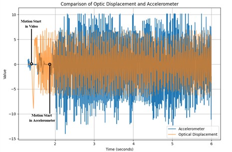
Upon further analysis, the primary cause of the observed performance degradation was identified as a temporal misalignment between vibration measurements and video frame motion. This discrepancy stemmed from inherent asynchrony in the data acquisition systems: the camera and accelerometer operated on distinct internal timing mechanisms during data collection. As depicted in Fig. 8, the optical flow-derived motion from the video frames deviates from the accelerometer-recorded vibrations, with a pronounced offset in their initial timestamps. This desynchronization led to erroneous correlations between the visual motion in frames and their corresponding vibration values, compromising the accuracy of subsequent analyses.

An initial corrective measure involved applying a fixed delay to the video recording to compensate for the temporal desynchronization. However, subsequent analysis revealed that the necessary delay exhibited significant variability across recordings, rendering this approach inconsistent and unreliable. Consequently, a more robust and adaptive synchronization methodology was deemed necessary to ensure precise temporal alignment.

Fig. 8Vibration measurement labeling error

3.2. Improved model

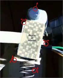
To improve prediction accuracy, a Region of Interest (ROI) is defined to isolate the vibrating object and suppress noise from background motion, as illustrated in Fig. 9. This spatial filtering ensures that only the most relevant pixel data contributes to the feature extraction process.

Fig. 9Motions outside of ROI

To resolve the desynchronization issue, an image preprocessing algorithm based on optical flow was implemented. This technique analyzes sequential frames in the video to detect and track pixel motion, effectively aligning video data with vibration measurements. The algorithm selects pixels located on textured regions or edges, where motion estimation is more reliable. Displacement is computed using the Euclidean Distance Formula by tracking pixel coordinates across frames. Velocity is then calculated by dividing displacement by the time interval, which remains constant at 1/125 seconds, corresponding to the 125-fps sampling rate. Acceleration is computed by evaluating the change in velocity across three consecutive frames. For frequency analysis, at least five frames are required to perform a Fast Fourier Transform (FFT), enabling the extraction of dominant vibration frequencies. This preprocessing strategy significantly improves temporal alignment between video and vibration data, ensuring more accurate and efficient feature extraction. A schematic representation of the optical flow algorithm is provided in Fig. 10.

To verify the effectiveness of this approach, the motion-derived values obtained through optical flow were compared against measurements from a calibrated vibration meter. The integration of optical flow notably reduced the number of input frames needed for accurate vibration analysis. Whereas the initial model required 30 or more frames to achieve reliable predictions, the optical flow-enhanced pipeline was able to compute displacement and velocity using only two frames, and acceleration and frequency using five frames. This optimization reduced the minimum frame requirement from 30 to 15, significantly enhancing computational efficiency without compromising prediction accuracy.

Fig. 10Optical flow validation flowchart

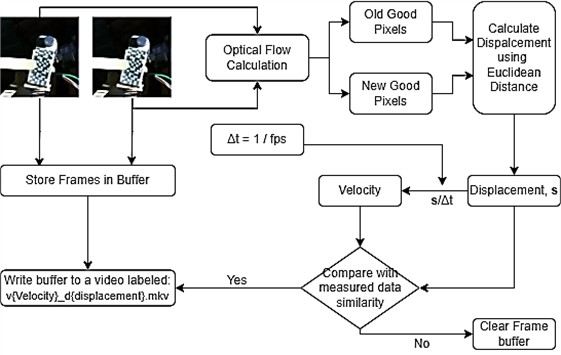
Table 2 presents the performance evaluation of the improved model, demonstrating significant enhancements across all metrics when tested on the same dataset. Among the vibration metrics, velocity exhibited the best performance, achieving a MAPE of 3.46 %, followed closely by displacement at 3.77 %. Acceleration ranked third with a MAPE of 4.53 %, while frequency recorded the highest error, with an MAPE of 11.76 %, indicating room for improvement. The RMSE values, which measure the average magnitude of errors, were 0.6979 for acceleration, 4.3467 for velocity, 0.0410 for displacement, and 4.5361 for frequency, highlighting the spread of prediction errors. The R² values, indicating the proportion of variance explained by the model, were 0.9809 for acceleration, 0.7949 for velocity, 0.7960 for displacement, and 0.8551 for frequency, reflecting the goodness of fit across these metrics.

One possible explanation for the performance disparity in frequency estimation is the lack of dataset variability. The collected frequency data is constrained to the natural frequency of the object, limiting the model’s exposure to diverse vibration patterns. This study focused on a single type of object with a constant mass and material composition, reducing the dataset’s generalizability. A thorough examination of the dataset revealed only four dominant vibration frequencies: 15.25 Hz, 30.50 Hz, 34.86 Hz, and 45.75 Hz. These frequencies align with values reported in studies on kinematic structure performance [34], which highlight common natural frequencies in machine vibrations.

The model's performance improved significantly following dataset augmentation with an expanded range of vibration frequencies and varied light illumination levels, as evidenced by the test results presented in Table 3. These enhancements, combined with optimizations across multiple model pipelines, yielded a 35.0 % reduction in MAPE from 11.76 % to 7.64 %, demonstrating improved accuracy in frequency metric prediction. The RMSE decreased substantially by 62.0 %, from 4.5361 to 1.7334, indicating markedly reduced prediction errors. Furthermore, the $R^2$ increased by 16.4 percentage points to 0.9954, showing near-perfect variance explanation. These improvements suggest that incorporating broader frequency spectra and illumination variability, along with pipeline optimization, effectively enhances the model’s generalization capability. While the current MAPE of 7.64 % may be acceptable for many applications, further refinement through techniques like weighted loss functions could potentially yield additional gains in prediction accuracy.

Fig. 11 presents the $R^2$ values for each measurement metric, evaluated using a dataset incorporating variable lighting conditions and an extended frequency range. The model demonstrates robust predictive capability, explaining over 80 % of the observed variance despite the presence of outliers.

Fig. 11R2 plot for all metrics

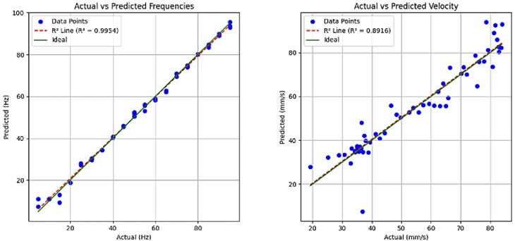
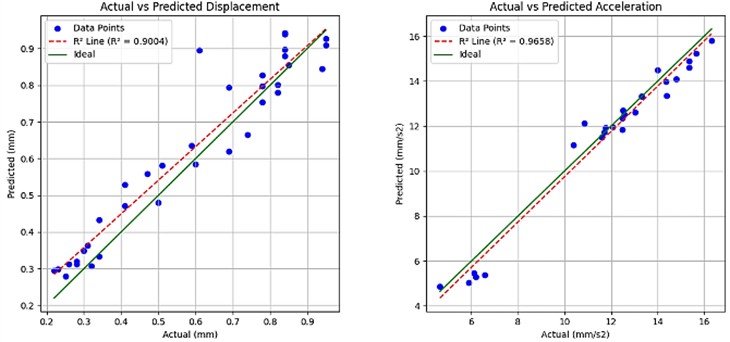
Detailed analysis of these outliers reveals systematic patterns in their distribution. The predominant cluster occurs at shutter speeds exceeding 700, where diminished light availability at the Raspberry Pi camera sensor significantly compromises feature extraction. Furthermore, the velocity metric exhibits a progressive increase in outlier frequency toward the upper range of measured values, attributable to motion blur artifacts when subject movement exceeds the camera's temporal resolution. This relationship between motion velocity and outlier prevalence is similarly reflected in the displacement metric, where higher displacement measurements demonstrate greater deviation from model predictions, consistent with the expected limitations of optical measurement under rapid motion conditions.

3.3. Effect of input size, network depth, distance to camera, and fiducial markers

Table 4 presents the MAPE values across different input resolutions and network depths, both with and without ROI cropping. The findings indicate that higher-resolution inputs generally lead to lower MAPE values, suggesting that increasing the input size enhances the model’s ability to extract meaningful vibration features. For instance, a resolution of 50×50 pixels consistently achieves a lower MAPE than 32×32 pixels. Increasing the number of layers improves performance, with deeper networks (four layers) consistently yielding lower MAPE values compared to shallower networks (two or three layers). This suggests that deeper architectures can better extract complex motion patterns from vibration data.

A critical observation is a dramatic reduction in error rates with ROI cropping, particularly for lower-resolution inputs. For example, at 50×50 pixels with four layers, MAPE drops from 56.37 % to just 5.93 % after applying optical flow validation and ROI cropping. This highlights the effectiveness of focusing on the core vibrating object, eliminating irrelevant background information, and improving model precision [36]. This analysis suggests that higher input resolutions, deeper networks, and ROI cropping significantly enhance performance. ROI cropping plays a crucial role in reducing error rates by isolating relevant motion areas.

As demonstrated in Table 5, the model exhibited significantly degraded performance when the fiducial marker was occluded, with prediction accuracy declining proportionally with increasing camera-to-object distance. This finding strongly suggests that the model has learned to utilize the marker as a key visual feature for motion estimation, effectively employing it to dynamically adjust the mm/pixel conversion parameters across varying distances. However, this capability introduces an important limitation: the model's performance is contingent upon the presence of the specific fiducial marker used during training. Experimental results indicate that variations in marker size or pattern would likely render the model ineffective, as it has not learned to generalize beyond the predefined marker characteristics. This dependency represents a significant constraint for practical applications requiring flexible marker configurations.

4.1. Maker dependence

A key limitation is the model’s reliance on fiducial markers for accurate motion estimation. As demonstrated in Table 5, prediction accuracy declined significantly when the marker was occluded, particularly at increased camera-to-object distances. This reliance constrains the system’s applicability in real-world scenarios where marker placement may be impractical or inconsistent. A potential solution involves employing feature detection on natural structures to serve as references for calibrating the distance-per-pixel parameter [37]. However, this approach may introduce challenges, such as elevated computational costs, rendering it impractical for real-time applications. Alternative approaches, such as stereo camera setups or single-camera systems with distance measurement sensors, offer potential solutions [38]. Given computational constraints, future efforts will first prioritize natural feature-based methods, which offer a balance between generalization and real-time feasibility, before exploring hardware-intensive solutions.

4.2. Data biases

The dataset used in this study was generated from a single-object, laboratory-scale setup with synthetic augmentation to increase frequency diversity. While effective for proof-of-concept validation, this introduces biases toward specific vibration patterns, lighting levels, and object characteristics. Such biases may reduce model robustness when applied to multi-component machinery or noisy industrial environments, where vibration signals are more complex and varied.

To address this, future work will expand the dataset in two stages: (1) collecting data from machines of varied shapes, materials, and operating conditions in controlled laboratory settings, and (2) collaborating with Sabah Electricity Utility Company to acquire data from real industrial systems. Additionally, optimizing hyperparameters, such as learning rates, length of sequence, and model architectures, will enhance performance and adaptability to diverse datasets [39-41]. To mitigate potential long-term data limitations, integrating recurrent neural networks (RNNs) into the model will enable stream learning, allowing continuous adaptation to new vibration patterns and environmental conditions [42]. Rigorous evaluation on diverse, unseen datasets from real-world applications, using metrics like mean absolute error for displacement and velocity, will be essential to quantify performance gaps and ensure robust generalization across complex scenarios.

4.3. Real-time application

In terms of performance, the model achieved an average inference time of 9.95 ms on workstation hardware but has yet to be benchmarked on embedded devices. Future work will focus on deployment to the Raspberry Pi 5, beginning with TensorFlow Lite (TFLite) conversion and quantization to reduce model size and latency. Lightweight architectures such as MobileNetV3 or EfficientNet-Lite for spatial feature extraction, combined with temporal modules like Temporal Convolutional Networks (TCNs), may further improve efficiency [43].

The goal is to approach real-time inference on edge hardware (e.g., <10 ms per frame), enabling continuous monitoring under typical industrial workloads. Profiling tools such as TensorFlow Lite Benchmark, perf, and hardware energy sensors will be used to quantify trade-offs in latency, power consumption, and accuracy. Multi-objective optimization methods (e.g., NSGA-II) may also be applied to balance competing requirements for accuracy and efficiency [44].

4.4. Frequency predictions

Compared to other vibration metrics, frequency predictions exhibited higher error, as shown in Tables 2 and 3. This is partly due to limited dataset variability: only four dominant natural frequencies were present in the collected data, restricting the model’s exposure to diverse vibration modes.

To improve temporal modeling, hybrid architectures such as CNN–LSTM, GRUs, or transformer-based models will be explored. CNN–LSTM and GRU architectures are well-suited for capturing sequential dependencies while remaining computationally efficient, making them candidates for edge deployment [45-47]. Transformer-based approaches may further enhance robustness by modeling long-range dependencies across frame sequences [48]. Future evaluations will benchmark these architectures against the current (2+1)D CNN backbone, focusing on accuracy, generalization, and real-time performance. Future work will explore these models, comparing their performance against the baseline model in terms of accuracy and computational efficiency, as outlined in the preceding subsection.

4.5. Safety-critical considerations

Beyond technical limitations, broader implications must also be considered, particularly when deploying ML-driven monitoring in safety-critical domains. The reliability of predictions may degrade under uncontrolled conditions such as occlusions, extreme lighting, or motion blur, potentially exceeding reported error margins. In high-stakes applications such as monitoring bridges, aircraft, or power grid infrastructure, such degradation could compromise timely fault detection.

Misclassifications pose additional risks. False negatives may allow undetected faults to progress into catastrophic failures, while false positives may trigger unnecessary maintenance, leading to downtime and economic losses. These risks highlight the need for human-in-the-loop oversight, with ML predictions serving as advisory tools supported by redundancy, fail-safe mechanisms, and cross-validation against conventional sensors.

Furthermore, ethical considerations arise from the use of video-based monitoring. Although this framework is intended for machine vibration analysis, deployment in shared environments could inadvertently capture sensitive or personally identifiable information. Robust privacy safeguards, including anonymization protocols and compliance with data protection regulations, are therefore essential.

To mitigate these risks, future development should prioritize dataset diversification to reduce bias, integrate uncertainty quantification to support decision-making, and adopt ethical deployment frameworks that emphasize transparency, accountability, and privacy. These measures will ensure that the proposed framework evolves into a responsible and trustworthy solution for predictive maintenance in safety-critical systems.