A new algorithm for finding the k shortest transport paths in dynamic stochastic networks

1. Introduction

Transportation is the lifeline of the national economy, and is the main carrier of pedestrian flow, material flow, capital flow and information flow in the socio-economic activities. In modern society, it is impossible to sustain economic development without efficient operation of the transportation system. However, with the dramatic increase of the amount of vehicles and the road traffic volume, the traffic congestion problem is increasingly serious, which has a serious impact on people’s daily travel and becomes a bottleneck restricting urban social and economic development. Traffic congestion and frequent traffic accidents have become increasingly common phenomena, which cause huge economic losses every year. How to make travel more efficiently has become the world’s problem. However, for the urban space is limited, in the face of the contradiction between the rigid supply of transport infrastructure and the flexible travel demand, it can’t completely solve the problem of traffic congestion through increasing investment in the construction of the transport infrastructure. So traffic guidance has become an effective way to solve traffic congestion problem. It can reduce blindness in travel, optimize traffic flow distribution and improve the efficiency of the urban road network through the selection of the shortest path, thus traffic congestion is eased.

Research on shortest path problem can be found in several existing literature, such as the literature [1-3]. The $K$ shortest paths (KSP) problem is a more general problem, wherein the KSP are calculated between a given source and destination node in a weighted graph [4]. The shortest path (lowest cost path) would normally be the preferred method from a given node to the destination node. When the shortest path between the two nodes is blocked, the second, the third, and the Kth shortest path must be determined as alternative paths. Several optimization problems can be expressed as the problem of calculating the shortest path between two nodes in a graph. The $K$ optimal solution is to calculate the KSP between two nodes. KSP algorithms for finding the KSP have been applied in various fields, such as transportation and communication systems as well as robot path planning [5-8]. A detailed discussion of the applications of the KSP algorithms was provided by Eppstein [4]. The KSP problem is attracting increasing attention in research.

To date, several research results have been obtained on the KSP problem [9-23]. The earliest literature on KSP dates back to Hoffman and Pavley (1959) [9]. Dreyfus (1969) [3] developed an efficient algorithm for solving KSP with a time complexity of $O\left(Kn\mathrm{l}\mathrm{o}\mathrm{g}n\right)$. Yen (1971) [10] proposed an algorithm with a time complexity of $O\left(K{n}^3\right)$. Lawler (1972) [11] proposed an algorithm with a time complexity of $O\left(kn\right(m+n\mathrm{l}\mathrm{o}\mathrm{g}n\left)\right)$. Katoh et al. (1982) [12], whose algorithm has a time complexity of $O\left(K\right(m+n\mathrm{l}\mathrm{o}\mathrm{g}n\left)\right)$, improved Yen’s algorithm. Eppstein (1998) [4] proposed an algorithm with $O(m+n\mathrm{l}\mathrm{o}\mathrm{g}n+kn)$, which significantly improved the efficiency of the KSP algorithm. However, the data structures adopted in his algorithm are complex. More literature related to the KSP can be found in the website established by Eppstein (http://liinwww.ira.uka.de/bibliography/Theory/k-path.html).

Studies on the KSP problem are limited to the static KSP problem. In real networks, the costs of network arcs and nodes are often dynamic and stochastic. The states of the arcs and nodes always change over time. The states cannot be determined before arriving at the arcs and nodes. Therefore, the costs of the shortest path are a function of stochastic events, which are subject to a certain probability distribution. Each arc and node is interrelated with neighboring arcs and nodes in a dynamic stochastic network. The events, which happen somewhere in the network, do not only affect an arc or a node of the network; they also tend to affect the arcs and nodes of neighboring regions. For example, in a traffic network, one unexpected traffic accident would not only block the traffic flow at the location of the accident, but it would also affect the traffic situations of neighboring regions or even block the neighboring intersections. Traditional KSP algorithms can solve the static KSP problem, but not the dynamic stochastic KSP problem.

The purpose of this paper is to study further the dynamic stochastic KSP problem (the paper is only concerned with the $K$ simple shortest path, i.e., loopless path), and to examine the use of genetic algorithm in solving the problem. The remaining parts of the paper are organized as follows. Section 2 provides the network symbols and the description of the KSP problem. The dynamic stochastic KSP problem is analyzed in Section 3. Section 4 explores a genetic algorithm for solving the dynamic stochastic KSP problem. The genetic operators are designed according to the characteristics of the network. Section 5 discusses the Nanjing City transportation network as the experimental object, and then verifies the KSP algorithm proposed in this paper. The last section summarizes the paper and discusses the future applications of the algorithm.

2. Notation

The network is described with graph $G=\{V,E,W\}$, which comprises three parts: a non-null node set $V=\{\mathrm{1,2},...,n\}$, one arc set $E_{v\times v}$ ($\left|E\right|=m$), and the set of cost (weight) functions $W$. Each node in the graph has a cost $W_i$, and each arc $e_{ij}=(i,j)\in E$ in the graph is endowed with a cost $W_{ij}$. The value of the cost is non-negative. Loops and multiple arcs are not allowed in the graph.

Fig. 1Network model

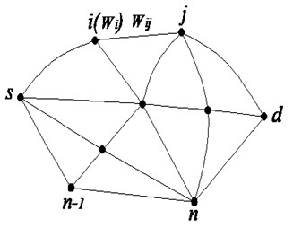
Definition 2.1 A path is an alternating sequence of limited nodes and arcs. A path from source node $s$ to destination node $d$can be expressed as $r(s=i,e_{ij},j,e_{jk},k,\cdots ,n=d)$. Circles are not allowed in the path.

The $K$ paths from the source node $s$ to destination node $d$ are denoted by $r_1\left(s,d\right),\mathrm{}{r}_2(s,d),\dots ,\mathrm{}{r}_k(s,d)$. The set $R(s,d)$ represents the collection of all paths from the source node $s$ to destination node $d$. The total cost of the path $r(s,d)$ is the sum of the costs of the nodes and the arcs through which the path passes. This cost is denoted by $l_r=\sum _{(i,j)\in r}{w}_{ij}+\sum w_i+\sum w_j$. If $w$ denotes stochastic variables, then $l_r$ is a stochastic variable as well.

3. Problem definition

The costs of arcs and nodes are deterministic in traditional KSP problems. However, the state of the arcs and nodes cannot be determined in advance. In the network $G$, the state of the nodes and arcs passed through by one path always changes over time, and the arcs and nodes are likely to be blocked under a certain probability. The arcs and nodes have two possible states, namely, blocked or unblocked. All arcs and nodes are interrelated. One blocked arc (or node) may cause other arcs (nodes) to be blocked. In such a case, using the probability model is more appropriate.

Definition 3.1 In a given network $G=\{V,E,W_e(t),W_i(t\left)\right\}$, $V$ is a non-empty set of nodes, $E$ is a set of arcs, $W_e\left(t\right)$ is the set of the cost functions of arcs, the arc cost is a stochastic process, $W_i\left(t\right)$ is the set of the cost functions of nodes, node cost is a time-dependent discrete stochastic variable, and the network $G$ is the dynamic stochastic network.

In a dynamic stochastic network, the arc cost can be modeled as a continuous stochastic process, which is denoted by $\left\{W_e\right(t),t\in T\}$, where $W_e\left(t\right)$ denotes the cost of arc $e$, $t$ is the time spent to arrive at the tail node of arc $e$, and $T$ is a continuous time parameter set. In $T=[t_0,t_m]$, i.e., $[t_0,t_m]$ is a closed interval of the interest time and $t\in [t_0,t_m]$, $t_0$ is the earliest departure time in the network, and $t_m$ is the endpoint of the interval. In $W_e\left(t\right)=\infty ,t>t_m,W_e\left(t\right)$ is a continuous stochastic variable for each instance $t$, and its probability density function is expressed as $f_{w_e}(w_e,t)$. When the flow of the arc rises to a certain level, the neighboring nodes may be blocked at a certain blockage probability, which is time-dependent. When one node $i$ is blocked, the cost of the node $W_i\left(t\right)$ is a positive value, whereas when the node is unblocked, its cost is 0.

When the volume and velocity of the arc flow rises, the volume and velocity of the node flow will also rise, and the blockage probability of nodes will become larger. The flow of the neighboring arc will be reassigned if one node is blocked. The arcs that are connected with the node will be blocked, and the cost of the arcs adjacent to the node will also change. These analyses indicate that the arcs and nodes in the network are interrelated. The $W_e\left(t\right)$ and $W_i\left(t\right)$ constitute a stochastic vector (variable):$V=\left\{W_{e_1}\right(t),\cdots ,W_{e_m}(t),W_1(t),\cdots ,W_n(t\left)\right\}$. The joint probability density function of this vector can be expressed as:

$f\left\{w_{e_1}\right(t),\cdots ,w_{e_m}(t),w_1(t),\cdots ,w_n(t\left)\right\}$.

The problem of calculating the KSP in a dynamic stochastic network is called the dynamic stochastic KSP problem. The main difference between dynamic stochastic KSP problems and the traditional KSP problems is the non-deterministic cost of arcs and nodes in the dynamic stochastic network. Only their statistic and probability distributions are known, i.e., $l_r$ is a stochastic variable. Solving the dynamic stochastic KSP problem involves finding the KSP among all the paths from the source node $s$ to the destination node $d$.

Given a path from the source node $s$ to the destination node $d:r\left(s=i,e_{ij},j,e_{jk},k,\dots ,n=d\right).$ The joint probability density function of this path is $f_r=\int \cdots \int f(w_{e_1},\cdots ,w_{e_m},w_1,\cdots ,w_n)d{w}_{e_q}\cdots d{w}_v$, where $e_q$ and $v$ are the arcs and nodes that the path does not pass through. Given $u$ paths from node $s$ to node $d$, the probability of the total costs of the path $r_i$ less than the other paths is $p_{r_i}\left(l_{r_i}\le l_{r_1},\cdots ,l_{r_i}\le l_{r_k},\cdots ,l_{r_i}\le l_{r_u}\right),k\ne i$. The following definition is derived from this equation.

Definition 3.2 The path $r$, which meets the condition,

$p_{\mathrm{r}}=\underset{i=\mathrm{1,2},\cdots ,u}{Max}{p}_{r_i}(l_{r_i}\le l_{r_1},\cdots ,l_{r_i}\le l_{r_k},\cdots ,l_{r_i}\le l_{r_u})$, is defined as the dynamic stochastic shortest path.

This path is the probabilistic shortest path with a probabilistic advantage over other paths. This path has the least expected cost and the lowest blockage probability among all paths. $p_{r_i}=\int \underset{G(l_{r_i}\le l_{r_1},\cdots ,l_{r_i}\le l_{r_u})}{\cdots }\int f(l_{r_i},\cdots ,l_{r_u})dL$, $f(l_{r_1},\cdots ,l_{r_u})$ is the joint probability density function of paths$\mathrm{}{r}_1,\cdots ,r_u$.

The dynamic stochastic KSP problem determines a set of $K$ (given an integer $K>$1) paths. The set is denoted as $R_K=\left\{r_1\right(s,d),r_2(s,d),\cdots ,r_k(s,d\left)\right\}$, where $R_K$ is a subset of the set $R(s,d)$, i.e., $R_K\subset R(s,d)$. The set $R_K$ meets the following conditions:

(1) $p_{r_{k-1}}>p_{r_k},k\in \left\{1,\cdots ,k\right\};$

(2) $p_{r_k}>p_r,r_k\in R_K$ and $r\in R-R_k;$

(3) In turn, these conditions determine the elements of the set $R_K$, i.e., the path $r_{k-1}$ is determined before the path $r_k$.

Calculating $p_r$ is extremely complex because large-scale complexity requires a large amount of computations. Thus, a compromise between accuracy and computability should be obtained. One cost ($W$) of the network at a certain moment always distributes in one continuous interval, not in different intervals. So we can derive the following property based on the knowledge of probability theory [24]:

Property 3.1 Given two stochastic variables $X$ and $Y$, $X$ distributes in one continuous interval, and the expectations of $X$ is $E\left(X\right)$; $Y$ distributes in one continuous interval, and the expectations of $Y$ is $E\left(Y\right)$. Then, $E\left(X\right)\le E\left(Y\right)\iff p\left(X\le Y\right)\ge 0.5E\left(X\right)$.

Proof: Assuming $E\left(X\right)\le E\left(Y\right)$, the result $p(X\le Y)\le 0.5$ is correct. However, this result is impossible. For example, given two independent stochastic variables $X$ and $Y$ with the following probability density functions:

The joint probability density function of $(X,Y)$ is then given as:

We can determine $E\left(X\right)=7<E\left(Y\right)=8$, but $p\left(X\le Y\right)=\underset{\Omega }{\iint }f(x,y)dxdy=0$. $625>0.5$ ($\Omega$ is the area that is composed of $6<x<8,$$4<y<12$ and $x\le y$). This result is contradictory to $p(X\le Y)\le 0.5.$ Thus, the conclusion $E\left(X\right)\le E\left(Y\right)\Rightarrow p(X\le Y)\ge 0.5$ is obtained. Similarly, $p(X\le Y)\ge 0.5\Rightarrow E\left(X\right)\le E\left(Y\right)$ is obtained.

Therefore,$E\left(X\right)\le E\left(Y\right)\iff p(X\le Y)\ge 0.5$.

The property shows that the path $X$ has probabilistic advantage over the path $Y$ because the expected cost of $X$ is less than that $Y$. Thus, we can find the path with maximum probabilistic advantage by comparing the expected costs of the paths. However, finding the path with probabilistic advantage in large-scale networks remains difficult because of the huge volume of computation. The analyses in the introduction indicate that the traditional KSP algorithms cannot find the KSP in dynamic stochastic networks. The dynamic stochastic KSP problem is an NP-hard problem. Thus, no existing polynomial time algorithm can be used. A new algorithm should be proposed to solve the problem. The genetic algorithm has excellent performance in searching spaces with large solutions, and can compromise between efficiency and accuracy. The genetic algorithm has been used in the shortest path problem and has achieved robust results [25-27]. The superiority of the genetic algorithm is proven in such problems. In this paper, we propose a dynamic stochastic KSP algorithm based on the genetic algorithm to solve the dynamic stochastic KSP problem.

4. Dynamic stochastic KSP genetic algorithm

4.1. Rules in chromosome encoding

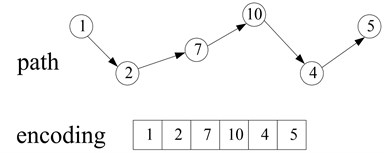
Chromosome encoding involves two modes: binary and real number encoding. The orderly aligned connected nodes in the network form a path. Adopting the ordered real number encoding mode to denote the paths in network is more reasonable. Therefore, the chromosome is naturally composed of a positive integer sequence that represents the nodes of a path. The genes of the chromosome are the nodes of the path, and each gene position represents a node position in the path.

The first gene of the chromosomes is the source node, whereas the last gene is the destination node. The lengths of the chromosomes are between 2 and $N$, where $N$ is the total number of the nodes in the network. The number of nodes of a path is not more than $N$ because loops are not allowed in the path. The length of the chromosome is variable because the numbers of the nodes of different paths are not the same. Thus, adopting the real number encoding mode, whereby the length is variable according to the number of the nodes of the path, is reasonable. This encoding mode is suitable when the number of nodes of different paths that connect the same source node and destination node are different. In such a situation, the fixed-length chromosome encoding mode will occupy a huge search space, which will reduce the efficiency of the algorithm. Figure 2 is given as an example. This figure shows a path from node 1 to node 5: 1 → 2 → 7 → 10 → 4 → 5 (directed network is used as an example to illustrate the KSP algorithm in this paper. The algorithm can be easily transplanted to the undirected network). Figure 3 shows the chromosome code.

Fig. 2One directed network

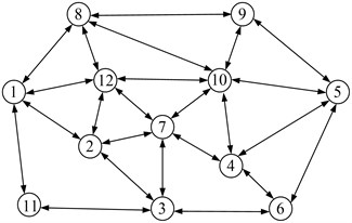
Fig. 3Example of chromosome encoding

4.4. Crossover operation

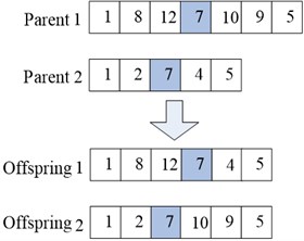
Another highly important component of the genetic algorithm is the crossover operation. A robust crossover operator can improve the search efficiency of a genetic algorithm. The path crossover operation exchanges two sub-paths of parent chromosomes. Population initialization causes the chromosomes to have the same source and destination nodes. The crossover operation is performed in selected chromosomes in two situations. First, when identical nodes are present in the two parent chromosomes (except the source and destination nodes), and the second, when no identical nodes are present.

In the first situation, the crossover operation is performed between identical nodes. In case of multiple identical nodes, one identical node is stochastically selected as the cross-location. Figure 4(a) illustrates the crossover operation (the network in Figure 2 is used as example).

Fig. 4Example of a crossover operation

a)

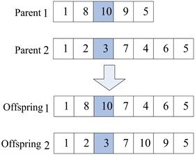
b)

Most real networks are incomplete networks in the second situation because illegal individuals can be generated in the crossover operation. Hence, the crossover operator needs to be improved to alter the illegal individuals. Further, using the network in Figure 2 as an example, given two paths (1 → 8 → 10 → 9 → 5 and 1 → 2 → 3 → 7 → 4 → 6 → 5) from source node 1 to destination node 5 selected as parent chromosomes, a pair of gene positions, e.g., {10, 3}, are stochastically selected as the location for the crossover operation. The offspring chromosome 2 that is generated during the crossover operation is an invalid path because no arc exists between nodes 3 and 9. Thus, the offspring needs to be altered. This procedure is accomplished through the heuristic method described in Section 4.2, whereby an effective path is established from node 3 to node 9 to turn offspring chromosome 2 into a legal path (shown in Figure 4(b)).

4.5. Mutation operation

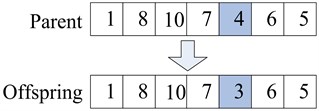
Path mutation operation generates another chromosome from one chromosome through mutation. Given the constraints of the topological relations in an incomplete network, operation mutation may generate illegal individuals. The mutation operator needs to be improved, thus, we designed the following mutation operator.

Step 1: The gene position to be mutated at a certain probability is stochastically selected.

Step 2: The selected gene and its adjacent genes compose a subpath, and another subpath is used to replace this subpath.

In illustrating the above steps, we continue to use the network in Figure 2 as example. Given node 4 as the gene selected for mutation in the chromosome, 1 → 8 → 10 → 7 → 4 → 6 → 5 is generated in the crossover operation described above, then node 4 is removed from the path, and another legal subpath is identified between nodes 7 and 6, as shown in Figure 5.

Fig. 5Example of a mutation operation

5. Computational experiment

We consider a transportation network described by a directed graph that is composed of a finite set of nodes and a finite set of arcs (Nanjing transportation network, Figure 6). In the Nanjing transportation network, each arc and node whose out-degrees are not zero are associated with a generalized cost, such as the travel-time or the distance or delay caused by blockage, and so on. This paper considers the travel-time of the arcs and the delay of the nodes as generalized cost without loss of generality. We assume that the travel-time of each arc is a continuous stochastic process and whose probability distribution depends on when to arrive at the tail node of the arc; further, we assume that the delay of each node is a discrete stochastic process and whose probability distribution depends on when to arrive at the node.

Fig. 6Nanjing traffic network (the right figure is one enlarged area)

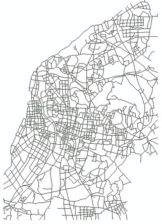
a)

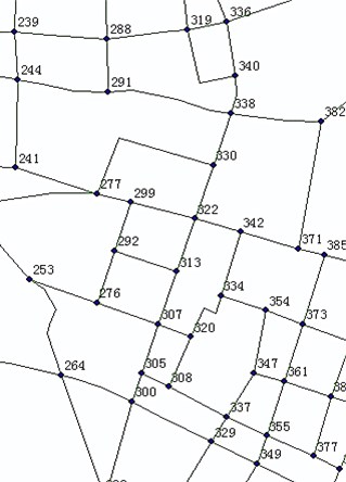
b)

The Nanjing transportation network has 2,668 arcs and 1,677 nodes. The rush hour (6:30 am to 8:30 am) was selected as the time interval for research. Due to the lack of statistical data on real-time traffic conditions, this paper built a simple dynamic stochastic network. The travel-time of the arcs and the delay of the nodes are expressed discretely; the selected time extent is divided into 10 sections, each composed of a 12 minute interval. The travel-time of each arc is subject to a certain normal distribution [29]. For instance, between 8:00 am and 8:30 am, the travel time of the arc from Jiuhua hotel to White Horse Park is subject to a normal distribution $N(3,22)$ (in minutes). The delay of each node is subject to a certain discrete distribution, e.g., the blockage probability of the intersection where Beijing East Road and Taiping Road intersects is 0.1, which causes a 4 minute delay, and thus, the expected delay of the intersection is 0.4 minute.

Using GIS software ArcGIS 10 as platform, the proposed algorithm is realized by simulation programming using C# development tools under the development environment VS. NET. The following genetic algorithm parameters are selected: population size $po{p}_{size}=$ 50, crossover probability$\mathrm{}{p}_c=$0.85, mutation probability$\mathrm{}{p}_m=$0.02, maximum evolution generations $Maxgen=$200, and $K=$5 (the five shortest paths are calculated). Nine pairs of source-destination nodes are selected stochastically from the transportation network to calculate the KSP. Experiment results are shown in Table 1. These results demonstrate convergent computational results, robust performance by the algorithm in convergence, and the average calculation time of less than 3 seconds, indicating high efficiency of the algorithm.

6. Conclusions

This paper studied the dynamic stochastic KSP problem. The dynamic and stochastic characteristics of a network were analyzed. The costs of the arcs and nodes were modeled as stochastic processes, and based on these, the concept of probabilistic KSP was proposed. The basic methods and strategies of applying the genetic algorithm to the KSP problem were explored; one dynamic stochastic KSP genetic algorithm was proposed to solve the dynamic stochastic KSP problem. The following conclusions were drawn:

1) The dynamic and stochastic characteristics of a network were not considered in the traditional deterministic KSP algorithms. However, most real networks, as well as the costs of arcs and nodes, are dynamic and stochastic. The principle of optimality proposed by Bellman is not suitable for solving the dynamic stochastic KSP problem.

2) The states of the arcs and nodes in the network are always interrelated. The interrelation of the arcs and nodes are more significant to the probabilistic shortest path model than to the traditional network model. Due to the complexity of large-scale networks, the amount of computation is too huge to calculate directly the $K$ probabilistic shortest paths. Based on the relation between the expected and the probabilistic advantage of the stochastic variable, we can find the probabilistic advantage shortest path by comparing the expectations.

3) The genetic algorithm has the ability to search a space of large solutions efficiently, and is very suitable in solving large-scale network combinatorial optimization problems. However, genetic operators should be improved according to the characteristics of the network. Experimental results demonstrate viable convergence and high efficiency of the proposed algorithm, which effectively solved the dynamic stochastic KSP problem. Thus, the genetic algorithm is an effective tool for solving such problems.

4) The model and algorithm proposed in this paper can be applied to communication networks, transportation networks, goods flow networks, and so on. For example, the algorithm can be used in intelligent transportation systems to guide vehicles dynamically, thus helping travelers reach their destinations quickly and easily. Therefore, the length of time that vehicles stay in the traffic network is reduced. The algorithm can significantly guide traffic flow and ease congested transportation.