Abstract
A bearing is the most common and vital element in the majority of rotating machinery. Condition monitoring and performance assessment of rolling bearing have recently attracted significant attention. This paper proposes a set of methodologies to realize the efficient health monitoring and assessment of rolling bearing. Considering the difficulties and disadvantages in detecting the fault signal of rolling bearing with background noise, this paper presents a method based on the Duffing oscillator and Hu’s moment invariant for health monitoring. The proposed method mainly combines the chaotic oscillator and moment invariant, fully utilizing the sensitivity of the former to detect the fault signal and taking the latter as a quantitative index for fault identification without the need for a qualitative artificial judgment on the Duffing oscillator phase trajectory map. To provide the optimal performance of Hu’s moment invariant in automatic recognition for the phase trajectory map, the influencing principle of different oscillator parameters was analyzed. Therefore, the health state of rolling bearing can be automatically monitored by quantitatively identifying the transition state of the phase trajectory map. A health assessment model was established to evaluate the health state of bearings. Wavelet packet transform was used to extract the features (approximate entropy) of bearing vibration signal, which were input into the self-organizing map (SOM) network. The health state of rolling bearings was then assessed using the SOM network and confidence values. A case study on health monitoring and assessment for rolling bearing was conducted to demonstrate the effectiveness and accuracy of the proposed methods.
1. Introduction
Rolling bearing is one of the most common fragile parts in mechanical equipment. According to statistics, this component is responsible for the 30 % of failures in rolling machines. Bearing failure is one of the foremost causes of breakdowns in rotating machinery, and such failure can be catastrophic, resulting in costly downtime. Therefore, bearing is important to numerous forms of machinery in manufacturing. Defect diagnosis and health assessment of rolling bearing have generated widespread interest in the area of manufacturing with a focus on preventing such failures. Previously proposed techniques are mainly based on vibration analysis [1-6]. However, the vibration signal of rolling bearing is always collected along with random noise. In terms of noise interference, traditional detection methods including spectral analysis [7], wavelet denoising [8], and mixture denoising diagnosis [9] aim to curb the noise through noise reduction and noise cancelling. These methods may achieve good results but may generate interference to useful signals to some degree.
Therefore, we propose an approach for the defect diagnosis and health monitoring of rolling bearing based on a chaotic oscillator, which exhibits excellent noise inhibition. The advantages of using a chaotic oscillator for signal detection is that it has nonlinear gain, high sensitivity to weak signals, bandwidth reduction, and a memory capacity useful for characterization. Signal detection with chaotic oscillator introduces a signal with a specific frequency as a periodic disturbance into the system and controls the system in the chaotic critical state. A large number of studies [10-15] on defect detection or diagnosis based on Duffing oscillator have been conducted, and satisfactory results have been achieved.
When a Duffing oscillator is used to detect a fault signal, the phase trajectory map will appear from the chaotic state to the large-scale periodic state. However, distinguishing the phase trajectory map or the time-domain waveform through visual observation is difficult, which may yield wrong conclusions. A number of studies [16, 17] have discussed the use of traditional or modified Hu’s moment invariants for the implementation of automatic visual pattern recognition and fault detection of industrial machinery.
Based on the aforementioned works, this study aims at combining moment invariant with Duffing oscillator to realize the health monitoring and diagnosis of rolling bearing. Different states of rolling bearing can be significantly identified during the transition of the phase trajectory map and critical moment invariant threshold between normal and faulty states. In this study, the effects of different parameter values, such as frequency of defect signal, sampling length, and external noise level, on the performance of moment invariant were determined. A health assessment model was used to evaluate the bearing health status.
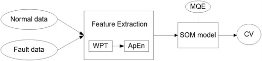
Fig. 1Procedure for the health monitoring and assessment of rolling bearing
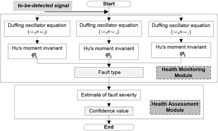
The proposed process is shown in Figure 1. Suppose that single-point faults occur, that is, the fault type is either one of inner-race, outer-race, and rolling element faults. First, three Duffing oscillators are set up according to the fault characteristic frequencies of the three fault types. The to-be-detected signal is then introduced to the three established Duffing oscillators, where , , and (, , represent the inner-race fault, outer-race fault, and rolling element angular frequencies, respectively). Hu’s moment invariants are then calculated by identifying the phase trajectories. The smallest among the three moment invariants , , and will be selected, and the corresponding pre-marked fault type is that which the introduced signal represents. Therefore, health monitoring is realized automatically based on Hu’s moment invariant calculation. Finally, the health assessment module is initiated after health monitoring. A health assessment model based on feature extraction and self-organizing map (SOM) is established. The health degree of rolling bearing, which is called confidence value, can be estimated through the established assessment model. Therefore, the health assessment of rolling bearing can be accomplished.
2. Principle of fault signal detection using chaotic Duffing oscillator
This paper employs the Duffing–Holmes equation for modeling. This equation provides the most straightforward and effective model for common rigid-forced vibration in mechanical systems. Numerous related studies on the characteristics of the equation have been conducted. For the Duffing–Holmes oscillator, a slight change in the parameters can result in an essential change in state. The Duffing–Holmes equation is written as follows:
where is the damping coefficient; and are the amplitude and the angular frequency of the internal periodic driving force, respectively; and is the nonlinear restoring force.
An equivalent set of two first-order non-autonomous equations is as follows:
After a time-scale transformation, a state equation can be obtained as Eq. (3):
When the to-be-detected periodic signal and noise are introduced into the oscillator, Eq. (3) is modified into Eq. (4) as:
where , , and are the amplitude, frequency, and phase of the to-be-detected periodic signal, respectively. represents other signals, including the random noise and invalid periodic components. A detection model was constructed for the periodic signal.
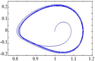
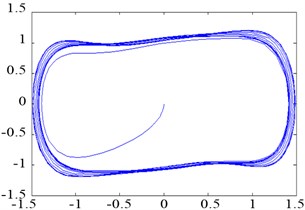
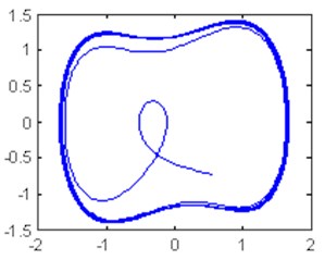
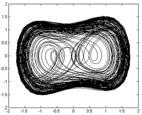
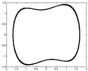
If is fixed and increases gradually from 0 to more than a certain threshold and continues increasing to exceed another threshold , then the time domain output and phase trajectory state of Duffing oscillator changes. The changing law in the phase plane is as follows: small-scale periodic state→chaotic state→large-scale periodic state. When 0.5, 2π∙100 rad/s, and the account (simulation) step 0.001, Eq. (3) can be solved by discretization using the fourth-order Runge–Kutta algorithm. To facilitate the observation on the transition of oscillator phase trajectories, the initial value {0, 0} was considered, and the first 100 data points were discarded. The corresponding phase trajectories are shown in Figure 2.
As shown in Figure 2, the Duffing oscillator is in the small-scale periodic state when 0.15, 1, in the chaotic state when 0.69, and in the large-scale periodic state when 0.7382. The driving force threshold (critical value), where the phase trajectory state of the Duffing oscillator shifts from the chaotic state to the large-scale periodic state, was 0.7381 based on repetitive simulation tests.
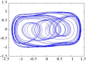
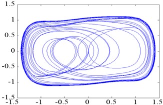
To verify the suitability of the Duffing oscillator for weak signal detection under strong noise disturbance, we set 0.7381 and kept the system in the critical chaotic state. By sequentially adding pure white Gaussian noise (as described in Eq. (4)) into the oscillator and increasing the standard deviation of the noise from 0.01 to 10, phase maps were generated, as shown in Figure 3 (a), (b), (c) and (d), respectively. The chaotic state did not shift into the large-scale state as the intensity of the added noise increased, which indicates that the state of the chaotic system can remain relatively steady under noise perturbation.
Fig. 2Phase trajectories of the Duffing oscillator with different parameters
a)0.15
b)0.69
c)0.7381
d)0.7382
Fig. 3Phase trajectory of the Duffing oscillator with pure noise: (a) σ= 0.01; (b) σ= 0.1; (c) σ= 1; and (d) σ= 10
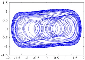
a)0.7381, 0.01
b)0.7381, 0.1
c)0.738, 1
d)0.7381, 10
3. Automatic identification of chaotic phase trajectories based on moment invariant
3.1. Hu’s moment invariant
For any 2-D image with a grey distribution function of the moment (sometimes called “raw moment”) of order is defined as:
where , 0, 1, 2, ....
The central moment is defined as:
where and are the components of the centroid.
During discrete transformation, the raw and central moments of are expressed as follows:
where , 0, 1, 2, ....
When variation occurs on the coordinate position of the image, changes correspondingly, whereas becomes sensitive to rotation with the translation invariant. In this study, the normalized central moment is:
where , and 2, 3, ....
If the image features are directly depicted using the raw and central moments, they will not be invariant to translation, rotation, or scale changes. However, the normalized central moment is invariant to translation as well as scale changes.
Hu [13] employed the results of the algebraic invariant theory and derived seven famous moment invariants using the second- and third-order central moments, which possess the invariant characteristics of translation, scale, and rotation in the case of continuous images. Hu’s moment invariants are defined as:
Relevant studies indicated that only the description of a 2-D object based on the second-order moment invariant is irrelevant to translation, rotation, and scale. Higher-order moments are highly sensitive to imaging errors, slight deformations, and other factors, such that the corresponding moment invariants cannot effectively recognize the object.
In Hu’s invariant set, only and are derived from the second-order moment invariant, whereas the other moments are based on the third-order moment invariant. The moment invariants and based on the second-order moment can be used to identify objects with significantly different shapes; otherwise, their moment invariants will be highly similar and thus difficult to recognize. In this paper, was used for the automatic diagnosis (i.e. health monitoring) of the object.
3.2. Automatic identification of phase trajectory map using moment invariant
As mentioned previously, was used as a quantitative index of the automatic diagnosis of the phase map in this paper. A large number of simulation works have shown that the phase trajectory maps in different states possess different which can achieve automatic identification by quantitatively recognizing the phase trajectory state.
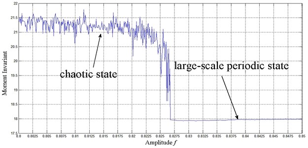
For Eq. (3), suppose that the sampling frequency is 1000 Hz, the sampling length is 5000, 2π∙60 rad/s, and ranges from 0.8 to 0.85 with a step size of 0.0001. The critical transition point (critical threshold point) can then be accurately derived as 0.8267, where the phase trajectory state changes from the chaotic to the large-scale periodic state. Figure 4 and Figure 5 show the change process of phase maps before and after the critical point. Figure 6 quantitatively reveals the change process of phase maps with ranging from 0.8 to 0.85.
Fig. 4Time domain waveform and phase trajectory map, f0= 0.8267; the Duffing oscillator is in the chaotic sate
a)
b)
By comparing the transition conditions of the phase trajectory map and Hu’s moment invariant in Figure 6, the moment invariant value was found to vary around 21 when the phase trajectory is in the chaotic state but stabilized at approximately 18 when the phase trajectory shifts from the chaotic to the large-scale periodic state.
Fig. 5Time domain waveform and phase trajectory map, f0= 0.8268; the Duffing oscillator is in the large-scale periodic state
a)
b)
3.3. Effect of different oscillator parameters on moment invariant
This section mainly discusses how Hu’s moment invariant changes in phase trajectory map under different parameters. Through the simulation, we determine the influence principle of different parameters, which provides the basis for the application of Hu’s moment invariant in the automatic recognition of phase trajectory maps.
Fig. 6Evolution of Hu’s moment invariant from chaotic state to large-scale periodic state
3.3.1. Effect of to-be-detected frequency on moment invariant
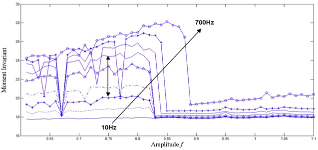
Suppose that the sampling rate is 1000 Hz, the sampling length is 5000, the amplitude of the internal periodic driving force is 0.6, and the amplitude of the external signal ranges from 0 to 0.5 with a step size of 0.01. The to-be-detected frequency was set as 10, 30, 60, 100, 200, 300, 400, 500, and 700 Hz sequentially, and the simulation result of Hu’s moment invariant in different phase trajectory maps along with the frequency’s variation was obtained, as shown in Figure 7.
Figure 7 shows that with an increase in the to-be-detected frequency, the inflection point where the phase trajectory map transfers from the chaotic to the large-scale state migrated. The chaotic oscillator was destroyed, such that weak signal detection cannot be realized. Therefore, the to-be-detected frequency must be approximately 10 Hz to 300 Hz for 1000 Hz sampling frequency to enable the chaotic oscillator to realize weak signal detection. If the to-be-detected frequency is high, the sampling frequency has to increase accordingly. As the to-be-detected frequency increases, Hu’s moment invariant of the chaotic oscillator in the chaotic state increases but remains at 18 in the large-scale state. Thus, the to-be-detected frequency should not be extremely low so that the accuracy of the moment invariant can be improved.
Fig. 7Hu’s moment invariant of phase trajectory map under different to-be-detected frequencies
3.3.2. Effect of sampling length on moment invariant
Suppose that the to-be-detected frequency is 60 Hz, the sampling rate is 1000 Hz, the amplitude of the internal periodic driving force is 0.6, and the amplitude of the external signal ranges from 0 to 0.5 with a step size of 0.01. The internal sampling length was set as 1, 2, 3, 4, 5, 6, 7, and 10 k sequentially. The changing behavior of Hu’s moment invariant with different values of sampling length in different phase trajectory maps was obtained, as shown in Figure 8.
Fig. 8Hu’s moment invariant of phase trajectory map at different sampling lengths
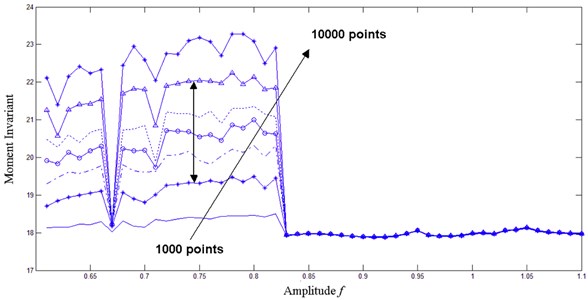
Figure 8 shows that when the sampling rate is 1000 Hz and the to-be-detected frequency is 60 Hz, the inflection point remains at the same value, without position changing. This phenomenon verifies the argument in section A. Moreover, the corresponding Hu’s moment invariant is smaller as the value of sampling length is smaller. Thus, the sampling length must not be too little if Hu’s moment invariant is used as a quantitative index. Otherwise, the judgment accuracy will be affected. Therefore, the best sampling length is more than 2000. Under a specified storage capacity of data acquisition equipment, higher sampling length will improve the performance of Hu’s moment invariant.
3.3.3. Effect of noise on moment invariant
Suppose that the to-be-detected frequency is 60 Hz, the sampling rate is 1000 Hz, the amplitude of the internal periodic driving force is 0.6, the amplitude of the external signal ranges from 0 to 0.5, and the step size is 0.01. Different intensity levels of white Gaussian noise with a mean of 0 and variance of were introduced into the oscillator. The variance was set as 0, 0.1, 0.2, 0.3, and 0.4, respectively. Under the same condition, the simulation result of Hu’s moment invariant in different phase trajectory maps with different noise levels was obtained, as denoted in Figure 9.
Fig. 9Hu’s moment invariant of phase trajectory map under different noise intensity
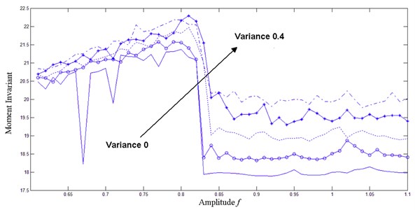
Chaotic oscillator has excellent inhibition for noise. However, as the surrounding noise signal increases, the oscillator map in large-scale periodic state changes, and the corresponding moment invariant improves continuously, thus diminishing regularity. When the system noise is strong, the availability of oscillator detection is relatively low. Therefore, the raw data should be processed before the Duffing oscillator and moment invariant are used for health monitoring.
3.4. Process of health assessment for rolling bearing
The health assessment procedure includes the following two steps.
3.4.1. Feature extraction
Approximate entropy (ApEn) is a measure of time series complexity from the perspective of reflecting the overall characteristics of signal [20] and has high anti-noise ability for random and ascertain signal. Only a short time-series is needed to calculate the ApEn of a signal. ApEn has been used with satisfactory results to assess mechanical equipment fault signals [21]. Thus, ApEn can be considered as a quantitative index of bearing defect severity. For ApEn calculation, the parameters of dimension m and tolerance value are quite crucial. According to the existing study [20, 21], ApEn values for all data sets were calculated with 2 and 0.25∙std(signal).
Wavelet packet transform (WPT) constructs a more sophisticated method for orthogonal decomposition based on multi-resolution analysis, which can divide the full frequency band of signal into multi-level, so that each band’s signal contains more elaborate information about the original signal. Therefore, wavelet packet decomposition is suitable to extract both low and high frequency characteristics.
After wavelet packet decomposition and reconstruction, the ApEn index of all bands reflecting signal characteristics will be calculated. If wavelet packet decomposition scale is too little, fault characteristics cannot be extracted effectively. However, large scale will also increase the dimension of characteristic vector. Therefore, during feature extraction, eight ApEn indexes from different frequency bands can be calculated using three-scale decomposition based on the characteristic of vibration signal.
3.4.2. SOM assessment model
SOM is an artificial neural network representing a multi-dimensional feature space in one- or two-dimensional space. SOM for health assessment can be trained only with normal operation data. In this study, SOM was trained iteratively using the aforementioned feature vectors. For each input vector, a best matching unit whose weight vector is closest to the input feature vector can be found in the SOM. The distance between the two vectors, which can be defined as the minimum quantization error (MQE), actually indicates the current operation status [22]. Hence, the performance degradation trend can be visualized by the trend of the MQE. Then, the MQE can be converted into confidence value (CV) ranging from 0 to 1 with some normalization approach, in which MQE increases while the CV decreases. Correspondingly, a suitable normalization function should have two characters: (1) CVs in different bearing faults should be close to 0 and approximate; (2) bearings close to the normal state have a CV close to 1.
As shown in Figure 10, normal bearing data was used to train SOM network after feature extraction with combined WPT and ApEn. Then, the fault feature vectors were input, which were also extracted using WPT and ApEn methods, into the trained SOM model. The health state of bearing can be assessed by CV values.
Fig. 10Flow chart of health assessment model
4. Case study. Application to health monitoring and assessment for rolling bearing
In this section, a case study on health monitoring and assessment of rolling bearing is presented. A group of vibration data from a bearing test rig was employed for verification. The test rig includes a 2-horsepower motor and a torque transducer/encoder. A deep groove testing bearing (6205-2RS JEM SKF) was installed on the motor. Table 1 shows the size parameters of the testing rolling bearing. Several types of single-point faults with the diameters of 0.007, 0.014, and 0.021 inches were introduced to the test bearings using electro-discharge machining, including inner ring, outer ring, and rolling element. The vibration data were collected using an accelerometer, which was installed at the 12 o’clock position of the drive-end of the motor housing by using a magnetic base.
The vibration data were collected at 12,000 samples per second, and the motor speed was 1772 rpm. Relative to background noise, the incipient fault signal is very weak. Suppose the contact between the rolling elements and inner/outer race is pure rolling, an impact will occur when the rolling elements pass through the local defect. The impact has a periodicity due to the uniform rotation of rolling bearing. The impact frequencies, i.e., characteristic frequencies, vary for the defects in different locations. In this study, the inner-race, out-race, and rolling element faults of the bearing were chosen for the verification of health monitoring. Table 2 shows that the fault characteristic frequency of the inner-race of the testing bearing was 5.4152 times as high as the rotation frequency. Therefore, the corresponding fault characteristic frequency was 159.9289 Hz. The outer-race and ball fault characteristic frequencies were 105.8731 and 139.2054 Hz, respectively.
Table 1Size parameters of the testing rolling bearing (Unit: inch)
Inside diameter | Outside diameter | Thickness | Ball diameter | Pitch diameter |
0.9843 | 2.0472 | 0.5906 | 0.3126 | 1.537 |
Table 2Defect frequencies (Unit: Hz)
Inner race | Outer race | Cage train | Rolling element |
5.4152 | 3.5848 | 0.39828 | 4.7135 |
: rotation frequency | |||
4.1. Health monitoring for rolling bearing with Duffing oscillator
4.1.1. Health monitoring for rolling bearing with inner-race defect
According to the characteristics of the testing bearings, the to-be-detected frequency should be in low frequency band. Thus, the acquired raw data was first re-sampled by decreasing the sampling rate from 12 KHz to 4 KHz. The signal was pre-processed with mean-removing and constant-proportional reduction to avoid introducing the high-amplitude vibration signal into the oscillator and destroying the oscillator state.
As shown in Table 2, the characteristic frequency (fault frequency) of the to-be-detected bearing was 159.9289 Hz. According to the analysis and optimization of different parameters for moment invariants in Section 3.3, 2π∙, 0.5, the sampling points 5000, and the sampling interval 0.0001. The amplitude of the initial internal periodic driving force is defined as 0.8267, which is the critical threshold and is obtained through several experiments. The Duffing oscillator used in this work is:
where is the to-be-detected normal or fault signals from the testing rolling bearings.
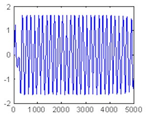
The above equations were solved using the fourth-order Runge–Kutta algorithm, and the result is shown in Figure 11.
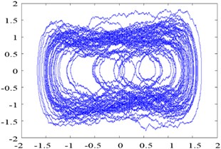
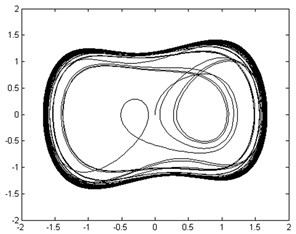
The moment invariant value of the phase trajectory map with chaotic state was approximately 20, as shown in Figure 11(a). However, the moment invariant value of the phase trajectory map with large-scale periodic state abruptly dropped and stabilized at approximately 18, as shown in Figure 11(b). Therefore, the rolling bearing is in the fault state, which has a moment invariant value of about 18. Hence, the health state (normal or faulty) of rolling bearings can be automatically distinguished by calculating the corresponding moment invariants of their phase trajectory maps.
Fig. 11Phase trajectories before and after adding inner-race fault signal: a) phase trajectory without inner-race fault signal in the chaotic state; b) phase trajectory with inner-race fault signal imported in the large-scale periodic state
a)
b)
4.1.2. Health monitoring for rolling bearing with outer-race defect
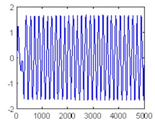
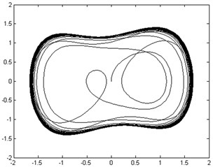
Based on the procedure described earlier, the outer-race fault data from the vibration signal were re-sampled at a sampling rate of 4 KHz and were then mean-removed and constant-proportionally reduced. The to-be-detected outer-race fault frequency was 105.8731 Hz, 2π∙105.8731, 0.5, 5000, the sampling interval 0.0001, and was 0.8267. Equation (10) was also solved using the fourth-order Runge–Kutta algorithm. The result is shown in Figure 12.
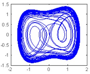
Fig. 12Phase trajectories before and after adding outer-race fault signal: a) phase trajectory without outer-race fault signal in the chaotic state; b) phase trajectory with outer-race fault signal imported in the large-scale periodic state
a)

b)
As shown in Figures 12 (a) and (b), the moment invariant value of the phase trajectory without outer-race fault signal added was 19.2 and 17.8 when the outer-race fault signal was imported. Thus, the normal and outer-race fault signals can be automatically distinguished by the corresponding moment invariant values.
4.1.3. Health monitoring for rolling bearing with rolling element defect
The raw vibration signal was re-sampled and then pre-processed with mean-removing and constant-proportional reduction before being input into the chaotic oscillator, where 2π∙139.2054, 0.5, 5000, 0.0001, and was 0.8267. The phase trajectories before and after adding fault signal are shown in Figure 13. The moment invariant values of phase trajectories with/without fault signal were 18.7 and 17.8, respectively.
Fig. 13Phase trajectories before and after adding rolling element fault signal: a) phase trajectory without rolling element fault signal in the chaotic state; b) phase trajectory with rolling element fault signal imported in the large-scale periodic state
a)
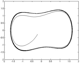
b)
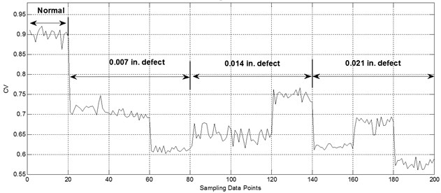
Fig. 14CV curve of rolling bearing with different fault severities and types
4.2. Health assessment for rolling bearing
According to the above-mentioned procedure in Section 2.4, normal bearing vibration signal was used first to train SOM network for 100 times. In this study, 20 normal signal samples were chosen, and eight ApEn values were calculated after wavelet packet decomposition for each training sample. Then, 180 fault vibration signal samples with three defect extents (0.007, 0.014, 0.021 inches), each of which includes inner-race, rolling element, and outer-race fault type, were introduced to the trained SOM model in sequence. Finally, the CVs curve indicating the performance degradation was obtained, as shown in Figure 14. The CVs of the first 20 points from the normal data were high, and the trend of the CV curve decreased as the fault severity increased. Therefore, health assessment for rolling bearing can be well achieved based on the SOM assessment model and CV.
5. Conclusions
The characteristics of chaotic Duffing oscillator and Hu’s moment invariants were analyzed, and the principle of the health monitoring method with combined Duffing oscillator and moment invariant was described. Moreover, the effects of different parameter values on the performance of moment invariant were determined, thus confirming the application conditions and limitations of the moment invariant. A health assessment model based on feature extraction with ApEn, WPT, and SOM network was presented. The increasing fault severity was correspondingly characterized by the decreasing CVs.
The case study for the health monitoring of rolling bearing showed that the value of moment invariant shifts rapidly and evidently as the state of phase trajectory map changes. Consequently, the moment invariant, as the quantitative criterion, can be used to identify the state of the phase map clearly and automatically without errors from qualitative eyeballing. Meanwhile, the SOM assessment model provides the desired result for bearing health state with CVs. The methods of health monitoring and assessment can generally enhance the automation level of fault detection and provide the reasonable health status for rolling bearing. Therefore, the methods have practical application value and can realize health monitoring and assessment for the entire life cycle of rolling bearing.
References
-
Ru-Qiang Li, Jin Chen, Xing Wu, Alfayo A. Alugongo. Fault diagnosis of rotating machinery based on SVD, FCM and RST. The International Journal of Advanced Manufacturing Technology, Vol. 27, Issue 1-2, 2005, p. 128-135.
-
Fan Sabirov, D. Suslov, Sergey Savinov. Diagnostics of spindle unit, model design and analysis. The International Journal of Advanced Manufacturing Technology, Vol. 62, Issue 9-12, 2012, p. 861-865.
-
Xinwen Niu, Limin Zhu, Han Ding. New statistical moments for the detection of defects in rolling element bearings. The International Journal of Advanced Manufacturing Technology, Vol. 26, Issue 11-12, 2005, p. 1268-1274.
-
Pavle Stepanic, Ilija V. Latinovic, Zeljko Djurovic. A new approach to detection of defects in rolling element bearings based on statistical pattern recognition. The International Journal of Advanced Manufacturing Technology, Vol. 45, Issue 1-2, 2009, p. 91-100.
-
J. H. Zhou, Z. W. Zhong, M. Luo, C. Shao. Wavelet-based correlation modelling for health assessment of fluid dynamic bearings in brushless DC motors. The International Journal of Advanced Manufacturing Technology, Vol. 41, Issue 5-6, 2009, p. 421-429.
-
Gang Yu, Changning Li, Jun Sun. Machine fault diagnosis based on Gaussian mixture model and its application. The International Journal of Advanced Manufacturing Technology, Vol. 48, Issue 1-4, 2010, p. 205-212.
-
Dron J. P., Bolaers F., Rasolofondraibe L. Improvement of the sensitivity of the scalar indicators (crest factor and kurtosis) using a de-noising method by spectral subtraction: application to the detection of defects in ball bearings. Journal of Sound and Vibration, Vol. 270, Issue 1-2, 2004, p. 61-73.
-
Hai Qiu, Jay Lee, Jing Lin, Gang Yu. Wavelet filter-based weak signature detection method and its application on rolling element bearing prognostics. Journal of Sound and Vibration, Vol. 289, Issue 4-5, 2006, p. 1066-1090.
-
Shao Y., Nezu K. Design of mixture de-noising for detecting faulty bearing signals. Journal of Sound and Vibration, Vol. 282, Issue 3-5, 2005, p. 899-917.
-
N. Q. Hu, X. S. Wen. The application of Duffing oscillator in characteristic signal detection of early fault. Journal of Sound and Vibration, Vol. 268, Issue 5, 2003, p. 917-931.
-
Chongsheng Li, Liangsheng Qu. Applications of chaotic oscillator in machinery fault diagnosis. Mechanical Systems and Signal Processing, Vol. 21, Issue 1, 2007, p. 257-269.
-
Wei Zhang, Bing-Ren Xiang. A Duffing oscillator algorithm to detect the weak chromatographic signal. Analytica Chimica Acta, Vol. 585, Issue 1, 2007, p. 55-59.
-
Zhen Zhao, Mingxing Jia, Fuli Wang, Shu Wang. Intermittent chaos and sliding window symbol sequence statistics-based early fault diagnosis for hydraulic pump on hydraulic tube tester. Mechanical Systems and Signal Processing, Vol. 23, Issue 5, 2009, p. 1573-1585.
-
Yunlong Cai, Chen Lu, Hongmei Liu. Incipient fault detection of rolling bearing based on Duffing oscillator. Proceedings of International Conference on Reliability, Maintenance and Safety, Chengdu, China, 2009, p. 858-863.
-
Abolfazl Jalilvand, Hossein Kazemi Kargar, Hadi Fotoohabadi. High impedance fault detection using Duffing oscillator and FIR filter. International Review of Electrical Engineering – Part B, Vol. 5, 2010, p. 1255-1265.
-
Devendran V., Hemalatha Thiagarajan, A. K. Santra Scene categorization using invariant moments and neural networks. Proceedings of the International Conference on Computational Intelligence and Multimedia Applications, IEEE Computer Society, Washington DC, USA, 2007, p. 164-168.
-
M. S. Al-Batah, N. A. Mat Isa, K. Z. Zamli, et al. A novel aggregate classification technique using moment invariants and cascaded multilayered perceptron network. International Journal of Mineral Processing, Vol. 92, Issue 1-2, 2009, p. 92-102.
-
Huang Z., Leng J. Analysis of Hu's moment invariants on image scaling and rotation. Proceedings of 2010 2nd International Conference on Computer Engineering and Technology (ICCET), Chengdu, China, 2010, p. 476-480.
-
M. K. Hu. Visual pattern recognition by moment invariants. IRE Transactions on Information Theory, Vol. 8, Issue 2, 1962, p. 179-187.
-
S. M. Pincus Approximate entropy as a measure of system complexity. Proceedings of the National Academy of Sciences of the United States of America, Vol. 88, Issue 6, 1991, p. 2297-2301.
-
R. Q. Yan, R. X. Gao. Approximate entropy as a diagnostic tool for machine health monitoring. Mechanical Systems and Signal Processing, Vol. 21, Issue 2, 2007, p. 824-839.
-
Hai Qiu, Jay Lee, Jing Lin, Gang Yu. Robust performance degradation assessment methods for enhanced rolling element bearing prognostics. Advanced Engineering Informatics, Vol. 17, Issue 3-4, 2003, p. 127-140.
About this article

This study is supported by the National Natural Science Foundation of China (Grant No. 61074083, 50705005) and by the Technology Foundation Program of National Defense (Grant No. Z132010B004).
