Dynamic characteristics of joint surface considering friction and vibration factors based on fractal theory

Li, Xiaopeng; Liang, Yamin; Zhao, Guanghui; Ju, Xing; Yang, Haotian

Journal of Vibroengineering

Browse Journal

Submit article

Published: 30 June 2013

Check for updates

Dynamic characteristics of joint surface considering friction and vibration factors based on fractal theory

Xiaopeng Li¹

Yamin Liang²

Guanghui Zhao³

Xing Ju⁴

Haotian Yang⁵

^{1, 2, 3, 4, 5}School of Mechanical Engineering &Automation, Northeastern University, China

Cite the article Download PDF

Downloads 1327

WoS Core Citations 9

Abstract

From the point of view of the micro-geometry, most joint surfaces are composed of the rough surfaces with the self-affine fractal characteristics. And the fractal characteristics have a large impact on the dynamic behaviors of the composite structures notably. In this paper the dynamic characteristics of the joint surface are discussed with the friction and vibration coupling effect considered based on fractal theory. Friction and vibration are caused by the rough surfaces. Firstly the expressions of the stiffness and damping model are obtained based on the fractal contact theory. Secondly the contact parameters of the joint surfaces are studied and analyzed with the contact surfaces replaced by the equivalent damping layer with the stiffness and damping model. Thirdly, based on the fractal contact theory, the contact pairs are established by ANSYS to simulate the effect of the characteristics of joint surfaces by the finite element method. Finally the natural frequency and model analysis obtained from theory and experiment of the composite beams are comparatively analyzed. The results show that the established stiffness and damping models are well suitable for the reality of the joint surface.

1. Introduction

In a view of microscopic geometry, most joint surfaces are composed of rough surfaces with self-affine fractal characteristics. In order to create a more accurate dynamic model of joint surfaces, the dynamic characteristics of joint surfaces should be well understood. Many new theories and contact models of joint surfaces are obtained, although the research of the dynamic characteristics largely depends on the classic theories which contain Hertz, G-W, and M-B [1-3]. The G-W statistical model with characteristic of elastic and plastic contact was put forward by Nayak [1]. Majumdar [2] presented the improved M-B model which contains the affine fractal features. Professor Tian [4] proposed a defect of the fractal model where the contact stiffness is an unconditional equation, and then he put forward the modified mathematical formula based on the M-B model. The elastic, elastic-plastic and plastic fractal models of the rough contact surface were established by Zhu [5], and the influence of the interface friction and the elastic-plastic deformation process of the materials are all considered. The research on the deformation characteristics of joint surfaces begins with the contact mechanics point [6-8]. Then the fractal models with the friction which are seldom studied by the dynamics theory [9-10] by now are established gradually [11-12].

Considering the friction of the joint surfaces, the fractal models of the contact stiffness and damping of joint surface are deduced based on the M-B contact model in this paper. Then the joint surface is replaced by the equivalent damping layer based on the obtained models in the process of simulation. The contents of the dynamic characteristics and the finite element analysis are expanded with the modal strain method, which can improve simulation credibility. Finally the reliability of the equivalent method is verified by comparing the results of the modal experiment with the equivalent damping method.

2. Fractal prediction models of the normal contact parameters of joint surface

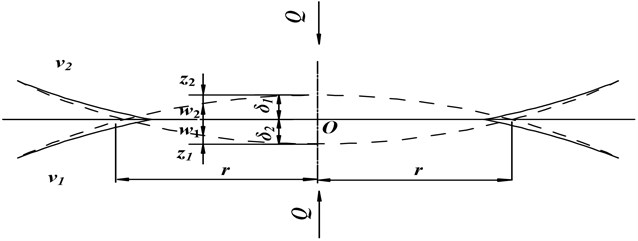
The friction between the contact surfaces of the mechanical joint surface makes the contact stress different from the classic Hertz solutions for different value and distribution. The influence of friction is ignored in the classic M-B fractal model. So it’s essential to modify the M-B model with the friction and establish the more accurate fractal model. The most basic theory of the contact surface is the Hertz theory and some fractal models are establied based on it. The section of the static contact deformation of two elastomers in Hertz theory is shown in Figure 1.

According to the Hertz theory, the real contact radius is:

1

r = {(\frac{3 Q R}{4 E})}^{1 / 3},

where $E = {[\frac{1 - v_{1}^{2}}{E_{1}} + \frac{1 - v_{2}^{2}}{E_{2}}]}^{- 1}$ is the equivalent elastic modulus. $Q$ is the contact force. $E_{1}$ , $E_{2}$ are the elastic modulus of two elastomers. $v_{1}$ and $v_{2}$ are the Poisson's ratios of the elastomers. And $R_{1}$ , $R_{2}$ are the curvature radiuses of the two elastomers, separately. The equivalent curvature radius of single peak is $R = {[\frac{1}{R_{1}} + \frac{1}{R_{2}}]}^{- 1}$ .

Based on the M-B fractal model, the mathematical model of the surface outline of the undeformed micro-bulge is expressed as Equation (2) [5]:

2

z (x) = G^{D - 1} a^{1 - 0.5 D} \cos (\frac{π x}{a^{0.5}}), - 0.5 a^{0.5} < x < 0.5 a^{0.5},

where $a$ is the actual contact area, $D$ is the fractal dimension, $G$ is the fractal scale coefficient.

Fig. 1The section of the static contact deformation of two elastomers

When $x =$ 0 in the Equation (2), the contact deformation of micro-bulge can be expressed as Equation (3):

3

δ = G^{D - 1} a^{1 - 0.5 D} .

Through Equation (2), curvature radius of elastomer can be obtained as shown in Equation (4):

4

R = \frac{a^{0.5 D} G^{1 - D}}{π} .

And also the relationship between $a$ , $δ$ and $a_{c}$ , $δ_{c}$ is shown in Equation (5):

5

\frac{δ_{c}}{δ} = {(\frac{a_{c}}{a})}^{1 - D} .

From the Reference [5] and other references, the relation of the biggest contact area ( $a_{m a x}$ ) and the distribution of the contact points ( $n (a)$ ) is:

6

n (a) = \frac{D}{2} ψ^{1 - 0.5 D} a_{m a x}^{0.5 D} a^{- 1 - 0.5 D}, 0 < a < a_{m a x},

where $ψ$ is fractal area expansion coefficient.

When the relative sliding is produced in the joint surfaces, the influence of surface friction on the critical deformation between the elastic and plastic state of micro-bulge must be considered. And it can be expressed as follows:

7

δ_{μ c} = {(\frac{3 π p_{μ}}{4 E})}^{2} R = {(\frac{3.3 π k_{μ} σ_{y}}{4 E})}^{2} R,

where $σ_{y}$ is the yield strength, $k_{μ}$ is the friction coefficient correction factor, $k_{μ} = 1 - 0.228 μ$ , $0 \leq μ \leq 0.3$ , $k_{μ} = 0.932 e^{- 1.58 (μ - 0.3)}$ , $0.3 \leq μ \leq 0.9$ . So the critical area between the elastic and plastic states of micro-bulge can be obtained through Equation (3), Equation (4) and Equation (5) expressed as Equation (8):

8

a_{μ c} = {(\frac{3.3 π^{0.5} k_{μ} σ_{y}}{4 E})}^{\frac{2}{1 - D}} G^{2} .

When the micro-bulge is in the elastic deformation state, according to the Hertz theory the normal contact stiffness of a single micro-bulge is:

9

k_{n} = 2 r E .

The elastic deformation will happen when the contact area is larger than the critical area, while the influnce of the friction is considered. Considering the distribution of the micro-bulge area between joint surfaces and the elastic deformation, the fractal model of the normal contact stiffness of the whole joint surfaces can be deviated based on the Equation (1), Equation (6) and Equation (9):

10

K_{n} = \frac{2 D}{1 - D} π^{- 0.5} ψ^{1 - 0.5 D} E (a_{m a x}^{0.5} - a_{m a x}^{0.5 D} {a_{μ c}}^{- 0.5 D + 0.5}) .

Then the dimensionless expression is:

11

K_{n}^{*} = \frac{2 D}{1 - D} π^{- 0.5} ψ^{1 - 0.5 D} ({a^{*}}_{m a x}^{0.5} - {a^{*}}_{m a x}^{0.5 D} {a^{*}}_{μ c}^{- 0.5 D + 0.5}) .

From Equation (11) it shows that the stiffness of the joint surfaces is combined with the critical area of elastic-plastic deformation in friction state. When the fractal characteristic parameters of joint surfaces, such as $D$ , $G$ and material elastic modulus ( $E$ ), are obtained, the contact stiffness of joint surfaces can be estimated. The accuracy of estimating the actual contact rigidity will be improved by this method.

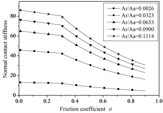
Then the influence of the friction coefficient on the normal damping of the joint surfaces can be obtained with the simulation software and the results are shown in Figure 2.

Form the Figure 2, the normal contact stiffness of joint surfaces continuously decreased with the increase of the friction coefficient. When the friction coefficient is less than 0.3, the dimensionless normal contact stiffness appears to have linear attenuation with the increase of the friction. And when the friction coefficient is larger than 0.3, the dimensionless normal contact stiffness appears to have the exponential attenuation with the increase of the friction coefficient, and the attenuation speed is reduced quickly with the increase of the actual combination area.

Based on the fractal theory we can study the expression of the contact stiffness and the influence of the friction coefficient on the stiffness from microcosmic angle. And the method to get the contact stiffness with the fractal theory would be improved.

Fig. 2The relationship between the normal contact stiffness and friction coefficient of joint surfaces

Now we will deduce the normal contact damping of the joint surfaces considering the effect of friction. When the elastic strain of single micro-bulge happened, the stored elastic energy can be obtained through integrating the contact load and deformation of single micro-bulge as Equation (12):

12

U_{e} = \int_{0}^{δ} P_{e} (δ) d δ = \int_{0}^{δ} \frac{4}{3} E R^{0.5} δ^{1.5} d δ = \frac{8}{15} E R^{0.5} δ^{2.5}, 0 < δ < δ_{μ c} .

And when the plastic strain of single micro-bulge happened, the irrecoverable deformation energy can be obtained through integrating the contact load and deformation of single micro-bulge:

13

U_{p} = \int_{δ_{μ c}}^{δ} P_{p} (a) d δ = \int_{δ_{μ c}}^{δ} K σ_{y} π R δ d δ = \frac{π}{2} K R σ_{y} (δ^{2} - δ_{μ c}^{2}), δ > δ_{μ c} .

According to Equation (2), and computing the integral of Equation (12) and Equation (13) for area respectively, we can obtain the stored elastic energy and the consumption of the plastic deformation of the whole joint surfaces in a contact process.

Then $U_{e}$ and $U_{p}$ are changed as Equation (14) and Equation (15):

14

U_{e} = \int_{a_{μ c}}^{a_{m a x}} U_{e} n (a) d a = \frac{4 D}{15 (2.5 - 1.5 D)} E π^{- 0.5} G^{2 (D - 1)} ψ^{1 - 0.5 D} a_{m a x}^{0.5 D} (a_{m a x}^{2.5 - 1.5 D} - a_{μ c}^{2.5 - 1.5 D}), (a_{m a x} > a_{μ c}),

15

U_{p} = \int_{0}^{a_{m a x}} U_{p} n (a) d a = \frac{D}{4 (2 - D)} K σ_{y} G^{D - 1} ψ^{1 - 0.5 D} a_{m a x}^{2 - 0.5 D} + \frac{1}{4} K σ_{y} G^{D - 1} ψ^{1 - 0.5 D} a_{m a x}^{- 0.5 D} a_{μ c}^{2}, (a_{m a x} \leq a_{μ c}) .

Damping factor ( $η$ ) is a kind of parameter that describes the damping characteristics of the structure or material and it is equal to the ratio of the dissipative energy and the storage of strain in a movement process:

16

η = \frac{U_{p} (a_{m a x} = a_{μ c})}{U_{e} (a_{m a x} > a_{μ c})} = \frac{15 \times (2.5 - 1.5 D) K}{16 D E π^{- 0.5} G^{D - 1}} \times \frac{σ_{y} a_{μ c}^{2 - 0.5 D} (\frac{D}{(2 - D)} + 1)}{a_{m a x}^{0.5 D} (a_{m a x}^{2.5 - 1.5 D} - a_{μ c}^{2.5 - 1.5 D})} .

When the structure is in resonance state, the relationship of the damping factor ( $η$ ), the normal contact damping ( $C_{n}$ ) and damping ratio ( $ξ$ ) is:

17

η = 2 ξ = \frac{2 C_{n}}{C_{c}},

where $C_{c}$ is the critical contact damping of joint surfaces. The $C_{n}$ can be obtained by Equation (17). And then with the simulation method the influence of the friction coefficient on the normal damping of joint surfaces can be studied, the results are shown in Figure 3.

Fig. 3The relationship between the damping factor and friction coefficient of joint surfaces

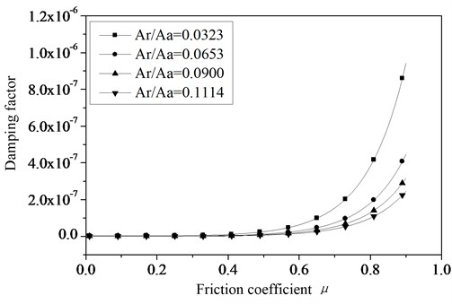
Form the Figure 3 the normal contact damping of the joint surfaces continuously increased with the increase of the friction coefficient. While the real contact area of the joint surfaces is becoming bigger, the friction coefficient is becoming bigger too. While the real contact area of the joint surfaces is smaller, the better damping performance will be obtained with changing the friction coefficient.

3. The fractal prediction model of the tangential contact parameters of joint surface

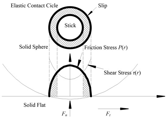
The former researches show that when the effect of dry friction is taken into consideration, the normal stress on the boundary of the contact circle is low, while the tangential stress is close to the infinite. So the boundary of the contact area will slip even under any size of the tangential load. The incomplete sliding will occur on joint surfaces when tangential load is smaller than the maximum static friction stress. In this condition the single point contact area can be divided into no slip region (adhesion circle with the radius $c$ ) and partly slip annular region of boundary. They are shown in Figure 4.

Fig. 4Tangential contact of micro-bulge with the effect of friction considered

The distribution of shear stress of adhesion region is assumed as follows:

18

τ_{s t i c k} (r^{'}) = - μ p_{0} \frac{c}{r} {(1 - {(\frac{r^{'}}{c})}^{2})}^{0.5}, 0 < r^{'} < c .

The distribution of the shear stress of partly slip region is:

19

τ_{s l i p} (r^{'}) = u p_{0} {(1 - {(\frac{r^{'}}{r})}^{2})}^{0.5}, c < r^{'} < r,

where $p_{0}$ is the maximum contact stress of the Hertz contact center, $p_{0} = 1.5 p_{m}$ , $p_{m}$ is the average contact pressure.

The displacement of the adhesion region $δ_{s t i c k}$ is:

20

δ_{s t i c k} = \frac{1}{4 G_{s}} r π μ p_{0} (1 - {(\frac{c}{r})}^{2}),

where $G_{s}$ is the equivalent shear modulus, $μ$ is the friction coefficient.

The total tangential stress of joint surfaces is:

21

Q_{t}^{'} = \frac{2}{3} π (τ_{2} r^{2} - τ_{1} c^{2}) = \frac{2 π r^{2}}{3} μ p_{0} (1 - {(\frac{c}{r})}^{3}),

22

\frac{c}{r} = {(1 - \frac{Q_{t}'}{\frac{2 μ π r^{2} p_{0}}{3}})}^{\frac{1}{3}} = {(1 - \frac{Q_{t}'}{μ Q})}^{\frac{1}{3}} .

The shear stiffness of the single contact point can be obtained with differential of $δ_{s t i c k}$ and taking Equation (21) into Equation (22). It is expressed as Equation (23):

23

k_{t}^{'} = \frac{8 G_{s} r (1 - {(\frac{c}{r})}^{3})}{3 (1 - {(\frac{c}{r})}^{2})} = \frac{4}{3} \frac{(1 - {(\frac{c}{r})}^{3})}{(1 - {(\frac{c}{r})}^{2})} k_{t} .

Only the plastic deformation of the contact point happened under the normal loading, the plastic flowing will happen along the tangential direction under the influence of the tangential forces. In this condition the ability to resist the shear deformation of the contact point is nearly lost. Hence, while obtaining the shear stiffness of joint surfaces, only the shear stiffness of the contact point where elastic deformation happened under the effect of the normal loading is taken into consideration. According to the distribution of the contact area of the fractal joint surfaces, the shear stiffness under the tangential force can be obtained as follows:

24

K_{t}^{*^{'}} = {(\frac{3}{4 π})}^{\frac{1}{3}} \frac{4 D}{1 - D} \frac{Q_{t}^{*}'}{1 - {(1 - Q_{t}^{*}')}^{\frac{2}{3}}} {Q_{n}^{*}}^{1 / 3} ψ^{1 - 0.5 D} \times {G^{*}}^{\frac{1 - D}{6}} {a^{*}}_{m a x}^{0.5 D} ({a^{*}}_{m a x}^{\frac{1 - D}{3}} - {a^{*}}_{μ c}^{\frac{1 - D}{3}}),

where $K_{t}^{' *} = K_{t}^{'} / G_{s} A_{a}^{0.5}$ is the dimensionless shear stiffness, $Q_{n}^{*} = Q_{n} / E A_{r}$ is the dimensionless normal loading, $Q_{t}^{*'} = Q_{t}^{'} / μ Q$ is the dimensionless tangential loading.

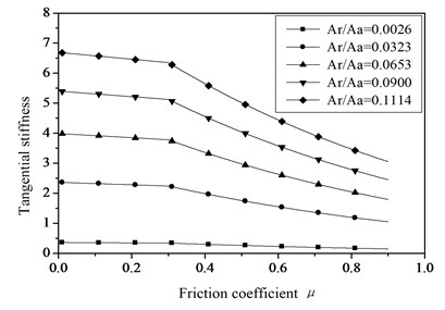
And then with the simulation method the influence of the friction coefficient on the tangential stiffness of joint surfaces can be studied, the results are shown in Figure 5.

The relationships between the tangential stiffness of joint surfaces and the friction factor with the fractal dimension $D =$ 1.25 and $D =$ 1.62 are shown in Figure 5. From the Figure 5 the tendence can be found, the tangential stiffness decreased with the friction factor increasing. But when $D =$ 1.25 the influence of friction factor on the tangential stiffness of joint surfaces will be reduced. At the same time there is no use in improving the tangential stiffness of the joint surfaces by only changing the friction factor.

Besides the friction generating from the slip of the joint surfaces will consume the energy of the system, which shows the dry friction damping characteristics. On the basis of this characteristic, the characteristics of tangential stiffness of the whole joint surfaces under the tangential cyclic load can be obtained.

Assume that the normal load on joint surfaces is $Q_{n}$ , the amplitude is $Q_{t}$ and the period of motion is $ϖ_{s}$ . Any two asperities are not only affected by the normal load $Q = a Q_{n} / A_{r}$ , but also by the tangential load $Q_{t}^{'} = a Q_{t} / A_{r}$ . When $Q_{t}^{'} < μ Q$ the two asperities are in the state of partial slip, the relationship between the tangential load and relative displacement is shown as ellipse.

Fig. 5The relationships of tangential stiffness and friction factor with different actual contact areas

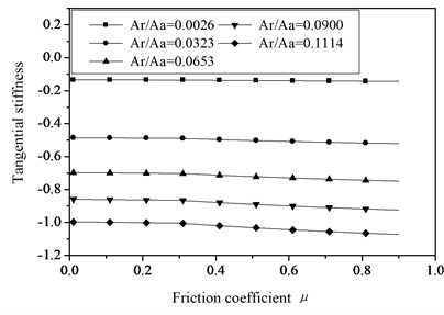
a) Fractal dimension $D =$ 1.25

b) Fractal dimension $D =$ 1.62

The energy consumed in one period of the whole joint surfaces is:

25

E_{d} = \int_{0}^{a m a x} e_{d} n (a) d a = \frac{1}{1.5 - 0.5 D} \frac{9 {(μ Q_{n})}^{2} π^{0.5} D}{5 G_{s} A_{r}^{2}} Λ ψ^{1 - 0.5 D} a_{m a x}^{1.5} .

Under the normal and tangential loading, the micro sliding area consuming the energy will be formed nearby to the contact point before the macro slipping of joint surfaces occurres. So the dry friction damping under the periodic tangential load can be replaced by the equivalent viscosity damping coefficient.

The equivalent viscosity damping coefficient of the dry friction damping is [6]:

26

C_{t e} = \frac{E_{d}}{π ϖ_{s} δ_{s t i c k}^{2}},

where $E_{d}$ is the work that the friction does in a whole period.

Substituting Equation (25) and Equation (20) into Equation (26), the expression of $C_{t e}$ is:

27

C_{t e} = \frac{64 G_{s} π^{0.5 - \frac{7}{3}} D}{ϖ_{s} (7.5 - 2.5 D) {(\frac{3}{4 E} \frac{Q_{n}}{A_{r}})}^{2 / 3}} \times \frac{Λ ψ^{1 - 0.5 D} a_{m a x}^{1.5}}{{(a^{1 + 0.5 D} G^{1 - D})}^{2 / 3}} .

If the contact radius is changed with the contact area changed, the dimensionless equivalent tangential damping factor of joint surfaces is expressed as follows:

28

C_{t e}^{*} = \frac{64 π^{0.5 - \frac{7}{3}} D}{{(\frac{3}{4})}^{2 / 3} (7.5 - 2.5 D) G^{*^{\frac{1 - D}{3}}}} \times \frac{Λ ψ^{1 - 0.5 D}}{Q_{n}^{*^{2 / 3}} a_{m a x}^{*^{\frac{2 D - 5}{6}}}},

where $G^{*} = G^{2} / A_{a}$ is the nondimensional parameter of the fractal dimension, $Q_{n}^{*} = 3 Q_{n} / 4 E A_{r}$ is the nondimensional parameter of the normal load, $a_{m a x}^{*} = a_{m a x} / A_{a}$ is the biggest single contact area of the nondimensional parameters, $Λ$ is the function about the friction coefficient of joint surfaces.

The factors in Equation (28) have a great influence on the contact characteristics of joint surfaces. And then with the simulation method the influence of the friction coefficient on the tangential damping ratio of joint surfaces can be studied, the results are shown in Figure 6.

Fig. 6The relationship between the tangential damping factor and the friction factor with different contact area

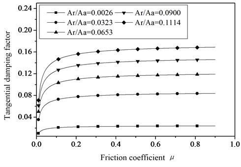
From the Figure 6 we can find that the tangential damping factor of joint surfaces becomes more stable with the friction coefficient increasing. The location of the break of $C_{t e}^{*} - μ$ curve will be affected by the size of the actual contact area. The critical friction factor $μ_{c}$ will move backwards as the actual contact area increases. The application of the theory of tangential damping factor of joint surfaces obtained in this paper is only applied to the state when micro partial slip occurred between joint surfaces.

4. Application and validation of the fractal contact models

When the machine is working, macro or micro displacement of joint surface will convert part of the mechanical energy into heat and noise consumption through friction, it essentially shows the damping characteristics. Based on the previous researches the joint surface can be equivalent to damping layer. Material constants of the damping layer can be determined based on the concept that the fractal contact stiffness is equal to strain energy. That’s to say, tangential parameters and normal paramenters obtained from the fractal model can be converted into the material properties of the damping layer. The damping layer is shown in Figure 7. The dynamic characteristics of joint surface are simulated with the finite element software by introducing the influence of the friction coefficient for the material properties of the layer.

By material mechanics, the power ( $W$ ) generated by the normal loading ( $Q$ ) in the elastic range is shown as follows:

29

W = \frac{Q^{2} h}{2 E A_{a}} = \frac{Q^{2}}{2 K_{n}} .

In the linear elastic range the strain energy of the equivalent damping layer of joint surfaces is:

30

V_{ε} = \frac{Q^{2} h}{2 E_{i} A_{a}} .

Due to the fact that the power ( $W$ ) generated by the external loading is equal to strain energy stored by the equivalent damping layer, equation is shown as follows:

31

E_{i} = \frac{K_{n} h}{A_{a}} .

In the same way the shear modulus ( $G_{i}$ ) of the material of the equivalent damping layer is shown as follows:

32

G_{i} = \frac{K_{t} h}{A_{a}} .

The relationship between the shear modulus ( $G_{i}$ ), elastic modulus ( $E_{i}$ ) and Poisson's ratio ( $v_{i}$ ) of the material of the equivalent damping layer is shown as follows:

33

ν_{i} = \frac{E_{i}}{2 G_{i}} - 1 .

Because the normal stiffness ( $K_{n}$ ) and the tangential stiffness ( $K_{t}$ ) of joint surfaces are the functions of the friction coefficient, Equations (30-32) show the relationship between the material coefficient of the layer and the friction coefficient. They also consider the influence of the friction coefficient, so they better match the engineering practice.

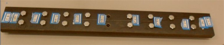
By using the stylus profile meter to measure the contact surface of the composite beams in Figure 8, the fractal dimension ( $D$ ) of its profilogram is 1.4781 and the fractal scale parameters ( $G$ ) are 0.00016.

Fig. 7The equivalent damping layer of joint surfaces

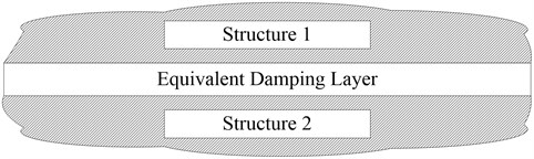
Fig. 8The composite beams for experiment

When the tightening torque of bolt is 4 Nm, by substituting the fractal parameters of steel plate ( $D$ ), ( $G$ ), elastic modulus ( $E$ ), Poisson's ratio ( $v$ ), density ( $ρ$ ) and friction coefficient ( $μ$ ) into Equation (10) and Equation (23), the normal contact stiffness ( $K_{n}$ ) and the tangential contact stiffness ( $K_{t}$ ) of joint surfaces are obtained. The parameters are summarized in Table 1.

Table 1The material constants and fractal parameters

$μ$	$E$ (Pa)	$ν$	$ρ$ (kg/m³)	$D$	$G$
0.12	2.1e11	0.3	7850	1.4781	0.00016

By putting these parameters into Equations (30), (31) and (32), the material constant of the equivalent damping layer is obtained. Considering the surface morphology of joint surfaces and the oxide layer and the plastic deformation layer by loading, the thickness of the equivalent damping layer is taken 8 mm. The material constants are summarized in Table 2.

Table 2The material constants of the equivalent damping layer

$E_{i}$ (Pa)	$ν_{i}$	$ρ$ (kg/m³)	$h$ (m)
5.5e8	0.35	7850	0.0008

According to the structure of the composite beams in order to accurately mesh the finite element model, which contains the top and the bottom steel plates and the equivalent damping layer, by ignoring the bolts the model is built. In the model the thickness of each steel plate is 6 mm, the equivalent damping layer is 0.8 mm, and each layer material is divided as 40×10×2 by the Solid-45 element with the simulation software, the total number of mesh points is 1200, it is shown in Figure 9. And each model shape and natural frequency are obtained through the method of Block Lanczos [13, 14] of modal analysis. The natural frequencies and loss factors of the composite beams processed by the equivalent damping layer are as summarized in Table 3.

Fig. 9The finite element model of the equivalent damping layer of the composite beams

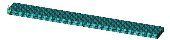
Table 3The natural frequency and loss factor of composite beams processed by equivalent damping layer

Modal order	1	2	3	4	5
Natural frequency (Hz)	374.5	912.2	1590	2384	3309
Loss factor	0.086	0.211	0.271	0.283	0.267

The relationship between the modal loss factor and the damping ratio of the system is linear under each resonance frequency. The damping characteristics of the composite beams can be demonstrated by the modal loss factor. The purpose of this experiment is to obtain the natural frequency and the damping ratio of the composite beams. The magnitude-frequency response curve of the composite beams is shown as in Figure 10. And the comparisons of the results of the equivalent damping layers and experiment are listed in Table 4.

Fig. 10The magnitude-frequency curve of the composite beams

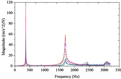
From the Table 4 modal parameters of each order of the composite beams with modal test are in agreement with the results, which are obtained by the finite element calculation method of equivalent damping layers with the influence of joint surfaces contact characteristics considered. The error of two kinds of results is about 5 %, and few may be close to 10 %. This method can provide the simulation value of modal loss factor related to structural damping. Above all the finite element calculation method of equivalent damping layers is used for the dynamics analysis of mechanical structure which considers the influence of joint surfaces.

Table 4Comparisons of the results of the equivalent damping layers and experiment

Modal order	Experimental natural frequency	Equivalent damping layers	Error (%)	Modal experiment damping ratio (%)	Equivalent damping layers
1	365	375	2.6	0.4	0.09
2	897	912	1.7	1.2	0.21
3	1691	1590	6.0	1.1	0.27
4	2430	2384	1.9	1.4	0.28
5	3030	3309	9.2	1.5	0.27

5. Conclusions

Based on the M-B model, the fractal model of the normal contact stiffness of joint surfaces is studied considering the friction coefficient between joint surfaces. The fractal model of the normal contact damping and the tangential contact stiffness is established based on the concept of modal loss factor. The fractal model of the tangential contact damping based on the equivalent treatment method of the friction damping is obtained when the surface is in the sliding state. After obtaining a fractal prediction model of the contact parameters of joint surfaces, this paper studies the influence of the friction coefficient on the contact stiffness and damping with simulation method. The simulation results show that the fractal prediction model considering the friction coefficient is certainly right.

The joint surface of the composite beams is equivalent to a damping layer and through this way the material constant of the equivalent damping layer is gained. The modal analyses of the composite beams are made with the modal strain energy method and through this analysis each of natural frequencies and modal loss factors are also gained.

Finally the modal experiment of the composite beams is done, and the modal parameters of joint surfaces and the composite beam are gained. The error of the results between experiment and equivalent damping is very small, so it is feasible to simulate the joint surface with the equivalent method.

References

Ni Jun. A perspective review of CNC machine accuracy enhancement through real-time error compensation. China Mechanical Engineering, Vol. 8, Issue 1, 1997, p. 29-34.

Search CrossRef
Jianguo Yang, Yongqiang Ren, Weibin Zhu, et al. Research on on-line modeling method of thermal error compensation model for CNC machines. Chinese Journal of Mechanical Engineering, Vol. 39, Issue 3, 2003, p. 81-84.

Search CrossRef
Shiping Su. Study on the Methods of Precision Modeling and Error Compensation for Multi-Axis CNC Machine Tools. National University of Defense Technology, Beijing, 2002.

Search CrossRef
Xiaoli Li. Modeling and Compensation for the Comprehensive Geometric Errors of NC Machine Tools. Huazhong University of Science and Technology, Wuhan, 2006.

Search CrossRef
Huanlao Liu. Research on the Geometric Error Measurement and Error Compensation of the Numerical Control Machine Tools. Huazhong University of Science and Technology, Wuhan, 2005.

Search CrossRef
R. Hocken, A. J. Simpon, et al. Three dimensional metrology. Annals of the CIRP, Vol. 26, Issue 2, 1997, p. 403-408.

Search CrossRef
P. M. Ferreira, C. R. Liu. An analytical quadratic model for the geometric error of a machine tool. Journal of Manufacturing Systems, Vol. 5, Issue 1, 1986, p. 51-63.

Search CrossRef
S. Yang, J. Yuan, J. Ni. The improvement of thermal error modeling and compensation on machine tools by CMAC neural network. International Journal of Machine Tools and Manufacture, Vol. 36, Issue 4, 1996, p. 527-537.

Search CrossRef
G. Q. Chen, J. X. Yuan, J. Ni. A displacement measurement approach for machine geometric error assessment. International Journal of Machine Tools & Manufacture, Vol. 41, Issue 1, 2001, p. 149-161.

Search CrossRef
Zhiyong Qu, Weishan Chen, Yao Yu. Research on volumetric error identification of guide. Chinese Journal of Mechanical Engineering, Vol. 42, Issue 4, 2006, p. 201-205.

Search CrossRef
Youwu Liu, Libing Liu, Xiaosong Zhao, et al. Investigation of error compensation technology for NC machine tool. China Mechanical Engineering, Vol. 9, Issue 12, 1998, p. 48-52.

Search CrossRef
G. Zhang, R. Yang Ou, B. Lu. A displacement method for machine geometry calibration. Annals of the CIRP, Vol. 37, Issue 1, 1988, p. 515-518.

Search CrossRef
Grimes R. G., Lewis J. G., Simon H. D. A shifted block Lanczos algorithm for solving sparse symmetric generalized eigenproblems. SIAM Journal Matrix Analysis Applications, Vol. 15, Issue 1, 1994, p. 228-272.

Search CrossRef
Hongsong Zhang, Renxi Hu, Shiting Kang. ANSYS 13.0 Finite Element Analysis from Entry to the Master. China Machine Press, 2011, p. 296-318.

Search CrossRef

About this article

Received

05 March 2013

Accepted

03 June 2013

Published

30 June 2013

Keywords

joint surfaces

contact theory

fractal theory

mechanical dynamics

Acknowledgements

This paper is supported by the National Natural Science Foundation (51275079), Program for New Century Excellent Talents in University (NCET-10-0301) and Fundamental Research Funds for the Central Universities (N110403009).

This is an open access article distributed under the Creative Commons Attribution License, which permits unrestricted use, distribution, and reproduction in any medium, provided the original work is properly cited.