Effects of the dynamic vehicle-road interaction on the pavement vibration due to road traffic

1. Introduction

The road unevenness determines the ride comfort, possible damage to goods, and vehicle wear and safety on one hand, and pavement damage and environmental noise and vibrations on the other hand. Traffic induced vibrations are a common source of environmental nuisance as they may cause discomfort to people, malfunctioning of sensitive equipment, and damage to nearby buildings [1, 2] and road substructures such as pavement and subgrade [3, 4]. Thus, there is a strong desire to predict the traffic-induced pavement vibration accurately. One of the major concerns is the ability to evaluate the dynamic interaction between a moving vehicle and an uneven road. More and more numerical models have been proposed for the prediction of the traffic-induced road vibration.

Kargarnovin and Younesian [5, 6] investigated the Timshenko beam vibration generated by moving loads on the Pasternak visco-elastic half space and nonlinear visco-elastic half space successively. Using a simplified model of truck, Gillespie [7] studied the road vibration generated by truck dynamic loads. Lu and Yao [8] studied the dynamic stress and deformation of a layered road structure under vehicle traffic loads based on laboratory measurements and numerical calculations. In these works, the traffic loads were generally treated as a series of constant loads, and the road unevenness was neglected. In practice, however, during the operation of the traffic, the dynamic loads and vibrations may be caused by local road unevenness. In order to assess the effect of road unevenness on the vehicle vibrations, a statistical description of the global road unevenness by a power spectral density (PSD) function is considered [9, 10]. For local road unevenness with a known geometry such as a speed bump or speed table, a deterministic description of the road profile can be used to estimate the resulting ground-borne vibrations [11].

In consideration of the recently researches above, a more realistic dynamic vehicle-road coupling model is needed to investigate the pavement vibration caused by moving vehicles. The objective of this paper is to study the effects of the dynamic vehicle-road interaction on the pavement vibration due to road traffic. Research is focused on the composition characteristics of vehicle and the geometric unevenness of pavement, and by regarding the vehicle, pavement and subgrade as a whole system, a vehicle-uneven pavement-subgrade coupling model is proposed. The dynamic equilibrium equations of the coupling system are deduced by considering the unevenness, pavement deformation and compatible deformation. The analytical solutions of additional dynamic load and vertical displacement of the pavement are derived using the Fourier transform method. By employing fast Fourier transform (FFT), the numerical results are obtained and used to analyze the influence of the moving vehicle speed, the wavelength and magnitude of pavement unevenness and the pavement properties such as the Young’s modulus and thickness on the dynamic displacement response. Computed results show that two peaks of the vertical response can be observed with increase of the uneven pavement wavelength and the vehicle speed because of resonance of the coupling system. Therefore, it is important to control the pavement unevenness and vehicle speed to avoid resonance in the engineering practice.

2. Analytical solutions of the vehicle and pavement-subgrade system

2.1. Model and governing equations of the vehicle system

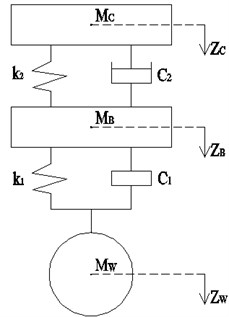
Experiments and analysis from vehicle research center show that a multi degrees-of-freedom (DOF) system, consisting of vehicle body, a bogie and a wheel, can be used to examine the vertical dynamic behavior of a moving vehicle [12]. Therefore, the multi degrees-of-freedom (DOF) system for vehicle (Fig. 1) is introduced in this paper. The vehicle is modeled as a two-body system but only vertical dynamics are considered. As shown in Fig. 1, symbols $M_C$, $M_B$ and $M_W$ denote the mass of the vehicle body, the bogie and the wheel, respectively. $k_2$and $c_2$denote the stiffness coefficient and damping coefficient of the secondary suspension per bogie, while that of the primary suspension per axle are denoted by $k_1$ and $c_1$.

Fig. 1Multi degrees-of-freedom (DOF) system of vehicle

The differential equilibrium equation of motion of forced damped vibrations for the two DOF system can be written as:

1

${\left[{\mathbf{M}}_V\right]}_{3\times 3}{\left[{\stackrel{..}{\mathbf{Z}}}_V\right]}_{3\times 1}+{\left[{\mathbf{C}}_V\right]}_{3\times 3}{\left[{\stackrel{.}{\mathbf{Z}}}_V\right]}_{3\times 1}+{\left[{\mathbf{K}}_V\right]}_{3\times 3}{\left[{\mathbf{Z}}_V\right]}_{3\times 1}=-{\left[\mathbf{B}\right]}_{3\times 1}\left\{\mathbf{P}\left(t\right)\right\},$

where $\left[{\mathbf{M}}_V\right]$, $\left[{\mathbf{C}}_V\right]$ and $\left[{\mathbf{K}}_V\right]$ ($V$ means vehicle) denote the mass, the damp and the stiffness matrices of the vehicle, $\left[{\mathbf{Z}}_V\right]$ the generalized displacement vector, $\left\{\mathbf{P}\left(t\right)\right\}$ the wheel-road force vector and $\left[\mathbf{B}\right]$ is a matrix of unit and zero elements. The minus sign before $\left\{\mathbf{P}\left(t\right)\right\}$ indicates that the positive wheel-road forces are of compression of the contact spring.

To derive the displacements due to a unit force of the vehicle at the wheel-road contact point, let $\left\{\mathbf{P}\left(t\right)\right\}=\left\{{\mathbf{P}}^{\text{'}}\left(\Omega \right)\right\}{e}^{i\Omega t}$ and $\left\{{\mathbf{Z}}_V\right(t\left)\right\}=\left\{{\mathbf{Z}}_V^{\mathbf{\text{'}}}\right(\Omega \left)\right\}{e}^{i\Omega t}$, where $\Omega$ denotes the angular frequency. Then Eq. (1) yields:

2

$\text{[}{\mathbf{Z}}_V^{\text{'}}\left(\Omega \right)\text{]}=-{\left(\left[{\mathbf{K}}_V\right]+\text{i}\Omega \left[{\mathbf{C}}_V\right]-{\Omega }^2\left[{\mathbf{M}}_V\right]\right)}^{-1}\left[\mathbf{B}\right]\left[{\mathbf{P}}^{\text{'}}\left(\Omega \right)\right],$

where $\left[{\mathbf{M}}_V\right]$, $\left[{\mathbf{Z}}_V\right]$, $\left[{\mathbf{K}}_V\right]$, $\left[{\mathbf{C}}_V\right]$ and $\left[\mathbf{B}\right]$ are detailed as follows:

${\left[{\mathbf{M}}_V\right]}_{3\times 3}=\text{diag}\left\{\begin{array}{ccc}{\mathbf{M}}_C& {\mathbf{M}}_B& {\mathbf{M}}_W\end{array}\right\},$

${\left[{\mathbf{Z}}_V\right]}_{3\times 1}={\left[\begin{array}{ccc}{\mathbf{Z}}_C& {\mathbf{Z}}_B& {\mathbf{Z}}_W\end{array}\right]}^T,$

${\left[{\mathbf{K}}_V\right]}_{3\times 3}=\left[\begin{array}{ccc}{k}_2& -k_2& 0\\ -k_2& k_2+k_1& -k_1\\ 0& -k_1& k_1\end{array}\right],$

${\left[{\mathbf{C}}_V\right]}_{3\times 3}=\left[\begin{array}{ccc}{c}_2& -c_2& 0\\ -c_2& c_2+c_1& -c_1\\ 0& -c_1& c_1\end{array}\right],$

${\left[\mathbf{B}\right]}_{3\times 1}={\left[\begin{array}{ccc}0& 0& 1\end{array}\right]}^T.$

The displacement vector of the wheel is part of that for the corresponding vehicle. Therefore, it may be written as:

3

$\left[{\mathbf{Z}}_W^{\text{'}}\left(\Omega \right)\right]={\left[\mathbf{B}\right]}^T\text{[}{\mathbf{Z}}_V^{\text{'}}\left(\Omega \right)\text{]}.$

In terms of Eqs. (2) and (3), the following relation is obtained:

4

$\left[{\mathbf{Z}}_W^{\text{'}}\left(\Omega \right)\right]=-{\left[\mathbf{B}\right]}^T{\left(\left[{\mathbf{K}}_V\right]+i\Omega \left[{\mathbf{C}}_V\right]-{\Omega }^2\left[{\mathbf{M}}_V\right]\right)}^{-1}\left[\mathbf{B}\right]\left[{\mathbf{P}}^{\text{'}}\left(\Omega \right)\right],$

let $\left[\mathbf{\vartheta }\right]={\left[\mathbf{B}\right]}^T{\left(\right[{\mathbf{K}}_V]+i\Omega [{\mathbf{C}}_V]-{\Omega }^2[{\mathbf{M}}_V\left]\right)}^{-1}\left[\mathbf{B}\right]$, $\left[\mathbf{\vartheta }\right]$denotes the receptance coefficient at the wheel-road contact point for the vehicle.

2.2. Model and governing equations of the pavement-subgrade system

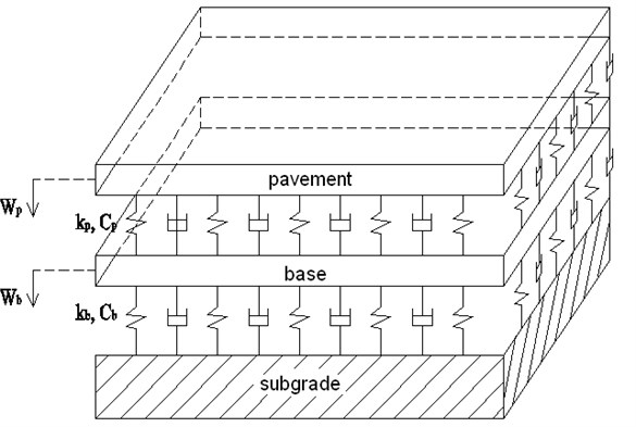
The model of pavement-subgrade system is shown in Fig. 2. A pavement-subgrade system described by two continuous layers of plates on elastic foundation is used. The pavement is modeled as an infinite plate satisfying Kirchhoff small-deflection thin-plate theory, as in Kim [13]. And the base layer is also modeled as an infinite plate ignoring bending stiffness. The contact condition between the layers is assumed to be viscoelastic. We introduce the rectangular Cartesian coordinate system $(x_1,y_1,z)$, which has its origin on the pavement surface with the $z$-axis pointing downwards. If one assumes the wheel-pavement force denoted by $\mathbf{P}(x_1,y_1,t)$, which is pointing downwards and located at $x_1=0$ when $t=0$. The load moves along the road at speed $V$.

Fig. 2The model of pavement-subgrade system

The governing equation for a pavement represented by a Kirchhoff plate is written as:

5

$D{\nabla }^2{\nabla }^2{W}_p\left(x_1-Vt,y_1,t\right)+k_p\left(W_p-W_b\right)+c_p\left(\frac{\partial W_p}{\partial t}-\frac{\partial W_b}{\partial t}\right)+{\rho }_p{h}_p\frac{{\partial }^2{W}_p}{\partial t^2}=P\left(x_1-Vt,y_1,t\right),$

in which ${\nabla }^2$ denotes the Laplacian operator, $W_p$ and $W_b$ are the vertical displacements of the pavement and the base layer, respectively, $D$ is the bending rigidity of the pavement, $k_p$ and $c_p$ are the stiffness coefficient and damping coefficient of the pavement, ${\rho }_p$ and $h_p$ are the density and thickness of the pavement.

The governing equation of the base layer can be written as:

6

${\rho }_b{h}_b\frac{{\partial }^2{W}_b\left(x_1-Vt,y_1,t\right)}{\partial t^2}-k_p\left(W_p-W_b\right)-c_p\left(\frac{\partial W_p}{\partial t}-\frac{\partial W_b}{\partial t}\right)+k_b{W}_b+c_b\frac{\partial W_b}{\partial t}=0,$

where $k_b$ is the stiffness coefficient of the base layer, $c_b$ is the damping coefficient of the base layer, ${\rho }_b$ and $h_b$ care the density and thickness of the base layer, respectively.

Suppose a vertical harmonic load moves along the road, in order to simplify the problem, a moving coordinate system $(x,y,z)$ is employed and the steady state displacement of the pavement is given by:

7

$W\left(x_1-Vt,y_1,t\right)=W\left(x,y\right)e^{i\Omega t},$

where $e$ is the exponential function, and $\Omega$ is the excitation frequency.

At this point, the double Fourier transform is introduced. Its direct and inverse forms are defined as follows:

8

$\left\{\begin{array}{l}\stackrel{-}{W}\left(\beta ,\gamma ,t\right)={\int }_{-\infty }^{+\infty }{\int }_{-\infty }^{\infty }W\left(x,y,t\right)e^{\text{-i(}\beta x+\gamma y)}\text{d}xdy,\\ W(x,y,t)=\frac{1}{4{\pi }^2}{\int }_{-\infty }^{+\infty }{\int }_{-\infty }^{\infty }\stackrel{-}{W}\left(\beta ,\gamma ,t\right)e^{\text{i(}\beta x+\gamma y)}\text{d}\beta d\gamma ,\end{array}\right.$

where $\beta$ and $\gamma$ are variations in the transformed domain corresponding to $x$ and $y$ in the physical domain.

The dynamic governing equations of the pavement and base layer can be solved by the steady state condition and Fourier transform. Using Eqs. (5)-(8), the expression of displacement of the pavement and the base layer in the transformed domain is obtained as:

9

${\stackrel{-}{W}}_p\left(\beta ,\gamma ,\Omega \right)=\frac{\stackrel{-}{P}\left(\beta ,\gamma ,\Omega \right)}{\left[D{\left({\beta }^2+{\gamma }^2\right)}^2-{\rho }_p{h}_p{\omega }^2+i\omega c_p+k_p\right]-\frac{{(i\omega c_p+k_p)}^2}{-{\rho }_b{h}_b{\omega }^2+i\omega c_p+k_p+k_b+i\omega c_b}},$

10

${\stackrel{-}{W}}_b\left(\beta ,\gamma ,\Omega \right)=\frac{i\omega c_p+k_p}{-{\rho }_b{h}_b{\omega }^2+i\omega c_p+k_p+k_b+i\omega c_b}\cdot {\stackrel{-}{W}}_p\left(\beta ,\gamma ,\Omega \right),$

where $\omega =\Omega -\beta V$.

To derive the receptance of the vehicle at the wheel-road contact point, a unit harmonic load is introduced as follows:

11

$P^e\left(x_1-Vt,y_1,t\right)=\delta \left(x_1-Vt\right)\delta \left(y\right)e^{i\Omega t}.$

By applying the double Fourier transform to Eq. (11), then substituting the transformed expression into Eqs. (7) and (9), the displacement of pavement in the time domain can be derived as follows:

12

$W_p^e\left(x,y,t\right)=\frac{1}{4{\pi }^2}{\int }_{-\infty }^{+\infty }{\int }_{-\infty }^{\infty }\frac{1}{\Delta }\cdot e^{i\left(\beta x+\gamma y\right)}d\beta d\gamma \cdot e^{i\Omega t},$

where $\Delta =[D{({\beta }^2+{\gamma }^2)}^2-{\rho }_p{h}_p{\omega }^2+i\omega c_p+k_p]-\frac{{(i\omega c_p+k_p)}^2}{-{\rho }_b{h}_b{\omega }^2+i\omega c_p+k_p+k_b+i\omega c_b}$.

After the displacement of pavement due to unit load is determined, it is rather straightforward to obtain the displacement of pavement under a moving load with arbitrary amplitude:

13

$W_p\left(x,y,t\right)=W_p^e\left(x,y,t\right)\cdot P^{\text{'}}\left(\Omega \right)=W_p^{\text{'}}\left(\Omega \right)\cdot P^{\text{'}}\left(\Omega \right)\cdot e^{i\Omega t},$

where $W_p^{\text{'}}\left(\Omega \right)=\frac{1}{4{\pi }^2}{\int }_{-\infty }^{+\infty }{\int }_{-\infty }^{\infty }\frac{1}{\Delta }\cdot e^{i(\beta x+\gamma y)}d\beta d\gamma$ is the receptance of the vehicle at the wheel-road contact point.

Once the displacement of pavement in the time domain is determined, the displacement of base layer can be obtained from Eq. (10) by means of the Fourier transform theorem.

3. Results and discussion

The numerical model is validated using field data from Lombaert and Degrande [14], who measured both the vehicle response and the soil response due to the passage of a Volvo FL6 truck on artificial road unevenness at vehicle speeds between 23 and 58 km/h. In this paper, only one axle of the vehicle is considered. Therefore, the following parameters of the truck are found following Lombaert and Degrande [14]: $M_C=\text{4500 kg}\text{,}$$M_B=\text{400 kg}\text{,}$$M_W=\text{150 kg}\text{,}$$k_2=\text{0.32}\text{×}{\text{10}}^{\text{6}}\text{N}/\text{m}$, $k_1=\text{3}\text{×}{\text{10}}^{\text{6}}\text{N/m}$, $c_2=\text{10050}\text{N·s/m}$, $c_1=\text{0}\text{N·s/m}$.

Two kinds of road unevenness can be distinguished: local road unevenness, which is only present at a limited distance along the road, and global road unevenness, which corresponds to the overall unevenness along the road. In Lombaert and Degrande‘s study [14], the artificial unevenness is taken as a traffic plateau with two ramps and a flat midsection. The unevenness height is equal to $H=\text{0.054 m}$, two slopes of length $l=\text{0.3 m}$ and a flat top part with a length $L=\text{1.3 m}$, the base length equals $L+2l=\text{1.9 m}$ and a width of 1 m. It is installed on a road with a smooth asphalt surface, using one three-ply board for each wheel path. In this study, a half-sine shape is considered to simulate the vertical profile of the artificial unevenness. Following Lombaert and Degrande [14], the magnitude and the wavelength of the unevenness are 0.054 m and 1.9 m, respectively.

The experimental road has a total width 6.20 m and is composed of an asphalt top layer and a foundation that is composed of a crushed stone layer and a crushed concrete layer. The parameters in this paper are the same as those estimated by Lombaert and Degrande [14]: the asphalt density ${\rho }_p=\text{2100}\text{kg/}{\text{m}}^{\text{3}}$ and a Poisson ratio $\mu =\text{0.33}$, the Young’s modulus of asphalt $E$ equals $\text{9150}\text{×}{\text{10}}^{\text{6}}\text{Pa}$, and the thickness of the asphalt layer $h_p=\text{0.15 m}$. The parameters of the crushed stone layer: ${\rho }_b=\text{2100}\text{kg/}{\text{m}}^{\text{3}}\text{,}$$h_b=\text{0.15 m}$, $k_p=\text{500}\text{×}{\text{10}}^{\text{6}}\text{N/m}$, and of the crushed concrete layer $k_b=\text{200}\text{×}{\text{10}}^{\text{6}}\text{N/m}$.

The truck’s axle accelerations were measured at the right-hand side of the vehicle by using 2 PCB accelerometers with a sensitivity of 0.1 V/g. Figs. 3 and 4 shows the time history of the predicted and the measured accelerations of the front axle for vehicle speeds of 30 and 58 km/h. The results are in good agreement with those obtained by Lombaert and Degrande [14], which indicates that the proposed model is useful in predicting the responses of vehicle and road structure.

In order to demonstrate some of the characteristics of the response of the system, a calculation is performed in this section by employing the fast Fourier transform. To compute the inverse transform accurately with a discrete transform, the integrals must be truncated at sufficiently high values to avoid distortion of the results, while the mesh of the calculated functions must be fine enough to well represent the details of the functions. Two typical vehicles denoted as medium truck and heavy truck, respectively, are introduced. The parameters for the trucks are listed in Table 1, corresponding to those used in Deng [12] and Sheng [15], and the parameters of pavement-subgrade system which are selected refer to Yao[16]. The parameters are selected according to Tables 1-2 if not being denoted in the figures.

Fig. 3Predicted (dash-dotted line) and measured (solid line) time history of the acceleration of the front axle for vehicle speeds V= 30 km/h

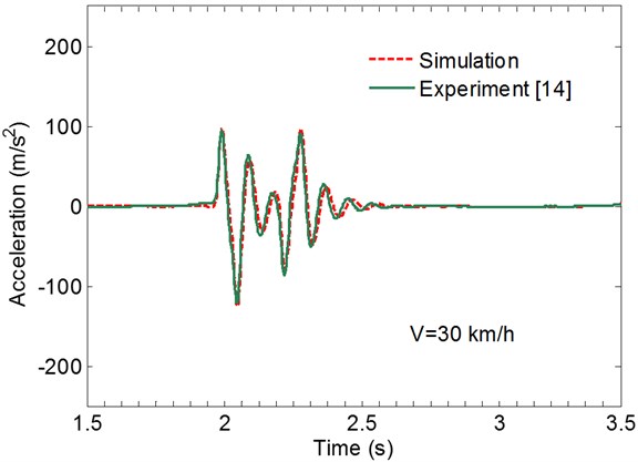
Fig. 4Predicted (dash-dotted line) and measured (solid line) time history of the acceleration of the front axle for vehicle speeds V= 58 km/h

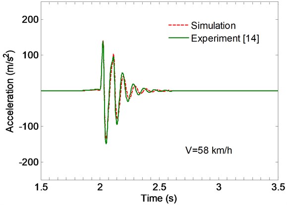
Fig. 5The effects of the wavelength of the pavement unevenness on the vertical displacement

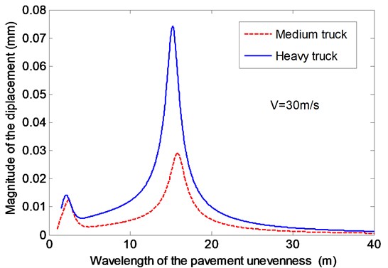
Fig. 6The effects of the magnitude of the pavement unevenness on the vertical displacement

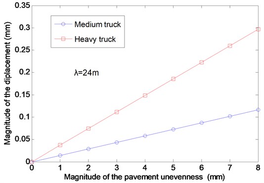
Fig. 7The effects of the vehicle speed on the vertical displacement for different thickness

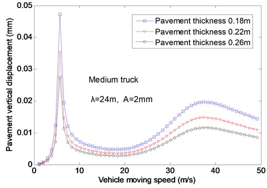
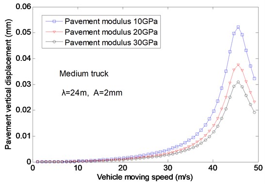
Fig. 8The effects of the vehicle speed on the vertical displacement for different modulus

The effects of the wavelength of the pavement unevenness on the vertical displacement of pavement are investigated in Fig. 5, which gives the results of medium truck and heavy truck, respectively. In Fig. 5, the magnitudes of the pavement displacement against the wavelength for vehicle speed $V=\text{30}\text{m/s}$ and the typical vehicles are presented. From Fig. 5, two peaks of the pavement displacement curves can be observed with increase of the wavelength because of resonance of the coupling system. It can also be seen that the magnitude of the pavement displacement increases as the wavelength increases and reaches the maximum values at two critical wavelengths of about 2.5 and 15, then decreases rapidly as the wavelength increases further. The vehicle types can affect the pavement displacements and the peak values apparently in that the weights and the natural frequencies of the two kinds of vehicles are different.

In Fig. 6, the variations of the magnitude of pavement displacement with the magnitude of pavement unevenness are presented for the medium truck and heavy truck, respectively. It can be seen from Fig. 6 that the magnitude of pavement displacement increases linearly as the magnitude of pavement unevenness increases, which indicates the pavement unevenness can affect the dynamic response apparently.

Fig. 7 presented the effects of the vehicle moving speed on the vertical displacement of pavement, where the medium truck is considered and the wavelength and the magnitude of the pavement unevenness are fixed at $\lambda =\text{3 m}$ and $A=\text{2 mm}$, respectively. As can be seen, there are two peaks of the pavement displacement curves with the increasing vehicle speed for pavement thickness$\mathrm{}{h}_p=\text{0.18 m,}$$h_p=\text{0.22 m}$ and $h_p=\text{0.26 m.}$ Two critical speeds, corresponding to the natural frequencies of the coupling system, are also observed. It is founded that the first peak values of the displacement are higher than the second ones for different pavement thickness. This reveals that the resonance between the primary suspension and the vehicle is more intensely than that between the secondary suspension and the vehicle. The variations of the pavement displacement with the vehicle moving speed are shown in Fig. 8, which gives the results of the wavelength $\lambda =\text{24 m}$ and the pavement modulus$\mathrm{}{E}_p=\text{10}\text{GPa}$, $E_p=\text{20}\text{GPa}$ and $E_p=\text{30}\text{GPa}$. It is found that only one peak of response curve can be observed when the vehicle speed increases because only one resonance occurs when the vehicle speed varying from 0 to 50 m/s, and the second resonance of the coupling system will occur at the moment of vehicle speed $V>\text{50 m/s}$.

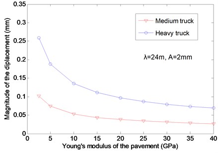
In order to investigate the influence of the pavement thickness and Young’s modulus on the pavement displacement more deeply, the variations of the displacement magnitudes with the pavement thickness and Young’s modulus are presented in Figs. 9 and 10. In these figures the wavelength and the magnitude of the pavement unevenness are fixed at $\lambda =\text{24}\text{m}$ and $A=\text{2}\text{mm}$, and the two kinds of vehicles are considered. It can be seen in Fig. 9 that the magnitude of the pavement displacement decreases by 80 % as the pavement thickness increases from 0.1 m to 0.3 m, and then gradually deceases to zero as the pavement thickness increases further. This result explains why this factor is so important in the design of pavements. It suggests disastrous effects on the pavement in the case of an under-estimated thickness and predicts inefficiency in the case of an over-estimated thickness. Finally, in Fig. 10, the effects of the Young’s modulus on the displacement magnitude are given. For low pavement modulus, the pavement displacement decreases sharply until the trend became constant as a larger modulus. This result implies that a reasonable pavement modulus should be chosen in the design of pavements.

Fig. 9The effects of the pavement thickness on the vertical displacement

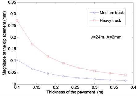
Fig. 10The effects of the pavement modulus on the vertical displacement

4. Conclusions

In this paper, a more realistic dynamic vehicle-road coupling model is proposed to investigate the effects of the dynamic vehicle-road interaction on the pavement response. The governing equations are solved by Fourier transform and the time-domain results are calculated by fast inverse Fourier transform. The effects of the wavelength and magnitude of pavement unevenness and the moving vehicle speed on the dynamic displacement response are investigated systematically. The influences of the pavement properties such as the Young’s modulus and thickness on the response are also studied. The main conclusions of this study can be summarized as follows:

(1) Two peaks of the pavement displacement curves can be observed with increase of the wavelength and the moving vehicle speed because of resonance of the coupling system. The resonance between the primary suspension and the vehicle is more intensely than that between the secondary suspension and the vehicle.

(2) The magnitude of pavement displacement increases linearly as the magnitude of pavement unevenness increases, which indicates the pavement unevenness can affect the dynamic response apparently.

(3) The displacement response of the pavement is sensitive to the variations in the pavement thickness and Young’s modulus. The numerical calculations showed that these two parameters are extremely important in the design of pavements and suggests potentially disastrous effects on the pavement in the case of an under-estimated thickness and suggests inefficiency in the case an over-estimated thickness.