Abstract
The radiation efficiencies of cylindrical and conical shells were investigated by using the statistical modal energy distribution analysis (SmEdA) and integrated FEM-SmEdA approaches. In cylindrical shell, three analytical algorithms were carried out, including SmEdA and two conventional approaches, i.e. the wave approach and the statistical energy analysis (SEA), and the results were compared with a former experimental one. SmEdA showed closest results with the experimental one, owing to its precise estimation of the coupling loss factors (CLF) which were further used to calculate the radiation efficiency. Furthermore, based on the analytical SmEdA, an integrated FEM-SmEdA algorithm is proposed. This hybrid method provided similar shell radiation efficiency for cylindrical shell, indicating its applicability in the analysis of complicated structures.
1. Introduction
The interaction between acoustic field and vibrating structure is often an important factor during structure design process. In particular, much attention has been paid on acoustic radiation efficiency. For example, lots of numerical studies have been performed to investigate the modal radiation efficiency of simply supported rectangular plate [1-5], and some also studied the boundary condition effect on the radiation efficiency for plate structure [6]. In addition to plate model, the cylindrical shell has also been paid much attention in the analysis of acoustic radiation efficiency, especially in the fields of aviation and marine. Earlier work by Manning and Maidanik pointed out that the extreme radiation efficiency at the ring frequency is due to the existence of the curvature [7]. Then in 1971, Szenchy first [8] presented an empirical formula of radiation efficiency for finite cylindrical shells based on statistical model. Recently, this method was extended to stiffened shells [9, 10]. However, the radiation characteristics were not well understood for thick shells, and the radiation efficiency was found to be dependent on geometries and boundary conditions [11, 12].
Wang and Lai [12] applied the coupling BEM/FEM method to analyze the sound radiation characteristics. However, for this approach, it is difficult to get accurate solution at high frequencies. While the modal radiation efficiency is based on massive calculation and the statistical empirical formula can not concisely predict the radiation efficiency of acoustically thick shells, it is necessary to propose another method to predict the radiation efficiency of general cylindrical shells.
In general, the structural damp effect is not taken into account when the wave theory is applied to calculate the coupling loss factors. However, SmEdA presented by Maxit and Guyader [13, 14] can be applied to conquer this drawback, and it can be directly used to calculate the energy transfer by using the dual formulation based on the modal displacement and force. Totaro and Dodard [15] calculated the coupling loss factors from the 2-D plate and Car frame structure to acoustic cavity, and they proved that this algorithm is valid for the acoustic-structural coupling problems.
In this paper, SmEdA is applied to calculate the coupling loss factor between the cylindrical shell and the acoustic cavity, and the radiation efficiency of the cylindrical shell is obtained by analyzing the relationship between the radiation efficiency and the coupling loss factor in the statistical energy analysis. Section 2 introduces the theoretical analysis of SmEdA. In Section 3, the Semi-analytical method obtained in Section 2 is validated by using the empirical formula of the radiation efficiency of the cylindrical shell proposed by Szechenyi. In Section 4, the coupling FEM and SmEdA is applied to calculate the structural radiation efficiency, and two numerical examples are presented to demonstrate the validity of the proposed algorithm for complicated practical problems.
2. Theory
2.1. Brief introduction of SmEdA
The SmEdA method is based on the dual formulation of modal shape-displacement [13], which considers an elastic-mechanical system as uncoupled-blocked subsystem 1 and uncoupled-free subsystem 2. The two uncoupled subsystems are characterized by stress mode shapes of subsystem 1 and displacement mode shapes of subsystem 2. In that case, the power balance between subsystem 2 and the th mode of subsystem 1 can be written as:
where , , , are, respectively, the modal input power, the modal damping, the modal frequency, the modal energy of the th mode of subsystem 1. is the number of modes of subsystem 2. is the modal coupling loss factor between the th mode in subsystem 1 and the qth mode in subsystem 2. Obviously the power dissipated by the th mode of subsystem 1 is given by , and the transmitted power from pth mode of subsystem 1 to th mode of subsystem 2 can be expressed as .
Since the modal energy equipartition assumption is introduced, the coupling loss factor between subsystem 1 and subsystem 2 is obtained by:
where and are, respectively, the center frequency and the number of modes of an octave band in subsystem 1. The Reissner principle is introduced to obtain the intermodal coupling factor (ICF) and the interaction modal work [13, 15]:
where and are the modal masses of the th mode of subsystem 1 and th mode of subsystem 2, respctively. is the displacement mode shape of th mode of subsystem 2, is the stress mode shape of the th mode of subsystem 1. is the outer normal vector component of subsystem 1.
Provided that the acoustic pressure is linear and of small amplitude, then the only degree of freedom (DOF) of the sound field is pressure. As a result, the characters of the vibro-acoustic system can be determined as following: the acoustic cavity can be described by modes of the uncoupled-blocked subsystem, and the structure by modes of the uncoupled-free subsystem. Because of the better representation of the boundary conditions, damping and modal overlap in the dual formulation, it is anticipated that the coupling modes theory based SmEdA method can provide more accurate analysis in low frequency than the aforementioned wave approach [15].
2.2. Description of the coupling system
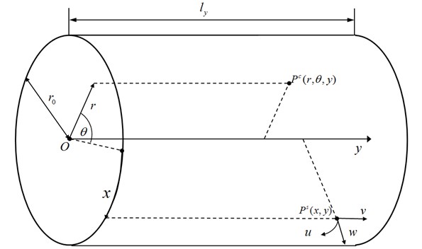
The coupling vibro-acoustic system is shown in Fig. 1. The cylinder thickness can be neglected in comparison with its radius and length A point on the surface of the cylinder is defined by co-ordinates giving its position circumferentially and axially. The displacements of the point are circumferentially, axially and radially outwards. A point in the cavity is defined by co-ordinates giving its position radially, circumferentially and axially.
Here we take the same boundary conditions as in reference [9]: simply supported at both ends for the cylindrical shell and complete sound absorption at both ends for the cavity. Hence the sound pressure is zero at the bulkheads in order to prevent radiation into the cavity.
Fig. 1Co-ordinate systems of the vibro-acoustic system
2.3. Modes of the uncoupled-free cylindrical shell
In this article, the Donnell equations are used to describe the stresses and displacements of the cylinder due to its simplicity and high accuracy for shells whose thickness is much smaller than its radius:
where is the tensile wave speed of the shell and is given by:
where , and are, respectively, Young's modulus, density and Poisson ratio of the shell material.
A wave motion with frequency and coupled , and motion can be represented by the following two forms:
where is the axial mode number and is the circumferential mode number. The wave number in the circumference direction can be given by:
Substituting Eq. (6) into Eq. (4) yields:
where:
For a non-zero solution, the determinant of the coefficient matrix must be zero:
and the boundary conditions for the simply-supported cylindrical shell are:
Substituting Eqs. (6) and (11) into Eq. (10) yields the characteristic equation of the eigenfrequencies as:
and the wave number in -direction is given by:
The three displacements could be decoupled by solving the characteristic equation due to the orthogonality of the co-ordinates. For each pair of and , consider the solution set with three positive roots derived from Eq. (12) as an eigenfrequency of the shell. Further research indicates that the eigenfrequencies of the torsional, longitudinal and bending modes, , and , are ranked in descending order, that is .
Cremer et al. [17] indicated that the in-plane modes of structures can not radiate power into acoustic cavities effectively. Hence only bending modes are considered in this article and will be used in place of for simplicity.
It can be seen from Eq. (6) that there are two forms of modes for the same pair of and , and the displacement mode shapes can be written as:
and the generalized modal mass is:
where superscript denotes the structure.
2.4. Modes of the uncoupled-blocked cavity
Consider the sound pressure of the acoustic cavity under a vibration frequency as:
where is the amplitude of sound pressure, is the pressure function.
For linear and small-disturbance acoustic field, the following wave equation must be satisfied:
where is the sound speed of the acoustic cavity. In cylindrical coordinates, equation (17) can be written as:
with the boundary conditions:
Substituting Eqs. (16) and (17) into Eq. (19) yields the pressure mode shape of the acoustic cavity:
where is the circumferential mode number. is the circumferential wave number. is the axial wave number. is the Bessel function of the first kind with the order and the argument .
It can be seen from Eq. (20) that must be satisfied for the rigid wall condition on the coupling surface. Since there are infinite zero points in the derivative of the Bessel function, numerous modes exist for arbitrary pair of and . The circumferential wave number of the modes are written as , where is the order of the zero point.
Consider that:
1. when , , only cosine-based mode shape exists;
2. when and , that makes and all the mode shapes are equal to zero.
We can finally derive the pressure mode shapes and the eigenfrequencies of the cavity:
The energy density of linear and small-disturbance acoustic field is:
where is the density of the acoustic cavity. Hence the modal kinetic energy of the cavity is given by:
Substituting Eq. (21) into Eq. (23) yields:
and the generalized modal mass of the cavity is:
where superscript denotes the acoustic cavity.
2.5. Radiation efficiency of the cylindrical shell
Radiation efficiency is used to represent the structure's ability of power radiation into the acoustic field. The total radiation efficiency, which is also called average radiation efficiency, is defined by:
where is the radiation resistance, is the spatially averaged mean square velocity of the structure, is the power radiated from the structure, is the area of the coupling surface.
The interaction modal work between th mode of cylindrical shell and th mode of the cavity can be given from Eq. (3b) by:
where is the displacement mode shape of the th mode of the cylindrical shell, is the pressure mode shape of the th mode of the cavity.
It is obvious that the shell's modes are decided by the combinations of mode number and , while the cavity's modes are decided by the combinations of mode number , and the zero point order . In the frequency band from to , is denoted by a number through the combinations of and , while is denoted by a number through the combinations of , and , is a number through the combinations of , and for . Then the number of the structure modes in the octave band is , while the number of the cavity modes is .
Substituting Eqs. (14) and (21) into Eq. (27) yields:
where the subscripts and represent the sine-sine and cosine-cosine modes coupling, respectively.
It can be seen from Eq. (28) that is nonzero only when , and the mode shape of the cavity and shell are both cosine function or sine function. Such pair of modes with nonzero-valued is called 'coupling pair', and pair of modes with zero-valued is called 'orthotropic pair' in this article.
We can obtain the intermodal coupling factor by substituting Eqs. (15), (25), (26) and (28) into Eq. (3a):
when :
otherwise:
Substituting Eq. (29) into Eq. (2) yields the coupling loss factor from the cavity to the cylindrical shell:
It can be seen from Eqs. (29) and (30) that only the coupling pairs of modes contribute to . According to classical SEA theory [16], the coupling loss factor from the shell to the cavity can be obtained through radiation efficiency by:
According to the reciprocity principle of SEA, the coupling loss factor from the cavity to the shell can be given by:
Cylindrical shell's radiation efficiency can be derived from Eqs. (30), (31) and (32) as:
It can be seen that the only parameters to which relates are the number of structural modes and the intermodal coupling factors, thus it is convenient and efficient to calculate the shell's radiation efficiency when the modal parameters of the structure and cavity in an interested octave band are acquired. These modal parameters can be obtained analytically for simple structures or numerically for complicated ones.
3. Comparison with conventional methods
Based on the aforementioned algorithm, the average radiation efficiency of a simply-supported cylindrical shell (as shown in Table 1) is taken as an example, and the calculated result is compared with that from conventional methods.
Table 1Cavity and shell characteristics
Cavity | Cylindrical shell | ||
(m) | 0.2515 | (m) | 0.2515 |
(m) | 0.63 | (m) | 0.63 |
(kg/m3) | 1.2 | (m) | 0.003 |
(m/s) | 340 | (kg/m3) | 7820 |
0.01 | (Pa) | 2.1e11 | |
0.3 | |||
0.01 | |||
3.1. Modes of subsystems
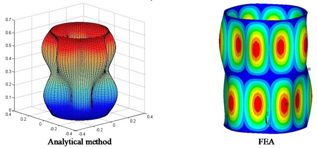
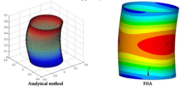
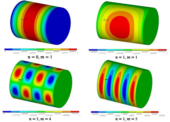
Eigenfrequencies of the cylindrical shell and the cavity below 8000 Hz are solved using the analytical methods, and FEA models of the subsystems are also built to get eigenfrequencies below 1800 Hz for comparison. Table 2 and Table 3 present eigenfrequencies of some typical modes of the shell and cavity obtained by the two methods, respectively. Figure 2 presents the comparison of some typical displacement mode shapes by the two methods. Figure 3(a) presents typical pressure mode shapes of the cavity on the coupling surface and Figure 3(b) presents typical pressure modes with same mode number , but different on the cross section at .
Table 2Eigenfrequencies of some typical shell modes
Analytical method / Hz | FEA method / Hz | Difference | ||
4 | 1 | 340.5499 | 340.481 | 0.02 % |
5 | 1 | 351.0907 | 351.275 | 0.05 % |
6 | 1 | 446.4968 | 447.25 | 0.2 % |
3 | 1 | 471.2864 | 471.232 | 0.01 % |
7 | 1 | 588.0045 | 589.689 | 0.3 % |
… | … | … | … | … |
11 | 4 | 1796.2 | 1790.5 | 0.3 % |
It should be noted that, when , two modes of the cavity or shell exist for arbitrary pair of , and with sine function or cosine function on the circumferential mode shape, and only one mode shape is presented here.
The good agreement between the modal results given by analytical method and FEM indicates that current analytical method is accurate and efficient enough for further analysis of the SmEdA.
Table 3Eigenfrequencies of some typical cavity modes
Analytical method / Hz | FEA method / Hz | Difference | |||
0 | 1 | 1 | 270 | 269.869 | 0.05 % |
1 | 1 | 1 | 476 | 479.411 | 0.7 % |
0 | 2 | 1 | 540 | 539.906 | 0.02 % |
1 | 2 | 1 | 667 | 669.726 | 0.4 % |
2 | 1 | 1 | 704 | 710.982 | 1 % |
… | … | … | … | … | … |
4 | 2 | 3 | 1797 | 1789.345 | 0.45 % |
3.2. Radiation efficiency of the cylindrical shell
Frequency band 630~8000 Hz is divided into twelve one-third octaves; the assignment of 30, 33 and 40 makes sure that no mode in the frequency band is missed during the analytical modal analysis. Table 4 presents the mode counts obtained by current method and SEA. It can be seen that there are obvious differences in low frequency range. For SEA, the empirical modal densities formula can produce a certain error as the frequency is low.
Table 4Mode counts of subsystems in 1/3rd octave band
Octave center frequency / Hz | Current method | SEA | ||
Shell | Cavity | Shell | Cavity | |
630 | 8 | 4 | 6 | 4 |
800 | 14 | 4 | 8 | 8 |
1000 | 16 | 10 | 12 | 14 |
1250 | 22 | 27 | 18 | 25 |
1600 | 30 | 39 | 26 | 47 |
2000 | 38 | 82 | 39 | 88 |
2500 | 70 | 159 | 61 | 165 |
3150 | 108 | 347 | 113 | 319 |
4000 | 110 | 608 | 119 | 628 |
5000 | 134 | 1244 | 135 | 1206 |
6300 | 178 | 2598 | 162 | 2367 |
8000 | 190 | 4800 | 200 | 4732 |
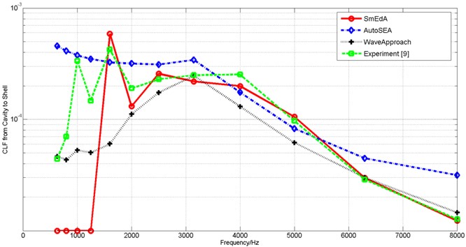
Figure 5 shows the coupling loss factors from the cavity to the shell calculated by wave approach [8], analytical SmEdA, experiment [9] and business software AutoSEA. Below 1250 Hz, wave length cannot be neglected compared with the structure dimension, and hence the wave field cannot be regarded as a reverberant one, which makes obvious difference between the results given by wave approach and experiment. For SmEdA method, no coupling pair of modes exists due to the small amount of modes in the octave and indicates that there is no energy transmitting between the shell and the cavity. The conflict between the results given by SmEdA and experiment indicates that the energy equipartition assumption is inaccurate in low frequency band. However, SmEdA method coincides the best with the experiment above 1250 Hz, not only reflecting the position of the maximum and the trend of , but also getting more and more closer to the experimental results as the frequency increases. On the other hand, the wave approach produces obvious difference almost in the whole frequency band and the business software AutoSEA, based on approximate formulas, gives the worst prediction, especially in the high frequency band.
Figure 6 presents the distribution of intermodal coupling factors in the 6300 Hz-centered octave band with the mode numbers , arranged in order according to the rank of modal frequencies. The distribution map shows a large number of cavity modes and shell modes, with only few coupling pairs of modes exist in this octave band. That is determined by the non-zero requirement of the and the integral orthogonality of the sine and cosine functions.
Fig. 2Typical mode shapes of the shell
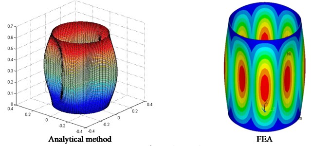
a) 4, 1
b) 5, 2
c) 1, 1
Fig. 3Typical mode shapes of the cavity
a) Mode shapes of the cavity on the coupling surface by FEA
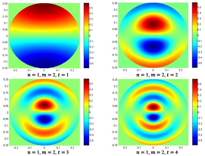
b) Mode shapes of the cavity on the cross section at 0.16 m by analytical method
Figure 7 presents the distribution of interaction modal work between cylindrical shell modes with mode number 1~5, 1 and cavity modes with same and but different zero point order of from 0 to 8000 Hz. It can be seen that decreases with the increase of and a typical cylindrical shell mode will transmit power into the cavity in more than one octave band. Take the coupling pair of 1, 1 as example, the eigenfrequency of the cylindrical shell mode is 1572 Hz in the 1600 Hz-centered octave band, there is no coupling cavity mode in the same octave, but is quite considerable for the cavity mode of 1 whose eigenfrequency is 476 Hz. In traditional modal analysis methods,only structural modes are considered in the frequency domain, while the cavity acoustic modal characteristics are rarely taken into account. In classical SEA, it is in a single octave band that the power balance theory between the subsystem-modes groups is set up, thus the current SmEdA algorithm should be more accurate than the others.
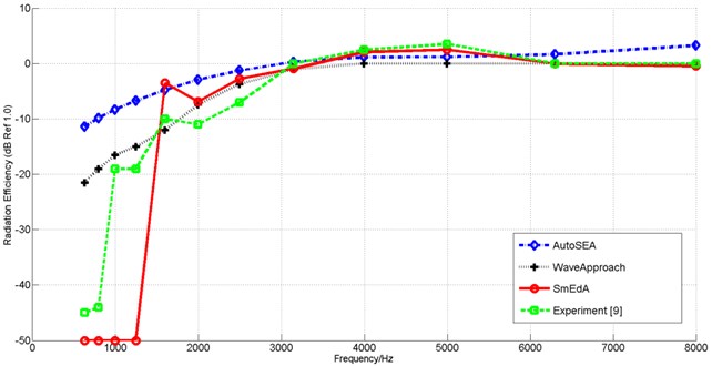
Figure 8 presents the radiation efficiencies given by the wave approach [8], the analytical SmEdA, experiment [9] and the business software AutoSEA. It can be seen that in the octave bands of 1000 Hz and 1250 Hz, the SmEdA-given is rather different from the three other approaches due to the lack of coupling pairs of modes. Notice the truth that the value of measured is very small below 800 Hz, the true value of can be considered to be zero in low frequency band in consideration of the inevitable errors caused by signal noise of the test devices and power radiated by the bulkheads during the experiment. Hence the SmEdA method agrees best with the experimental results while other methods are totally inapplicable in these octaves. Same situation occurs above 1250 Hz: the difference between results given by SmEdA and experiment is the smallest among all the numerical prediction methods. Not only the convergence of SmEdA-predicted to measured as frequency increases but also the exact positions of the extreme values demonstrate that the SmEdA approach is of most accuracy among all the predicting algorithms.
Fig. 5Coupling loss factor (CLF) from the cavity to the cylindrical shell
4. Application to engineering problems
Besides the high accuracy, another advantage of the SmEdA approach is the possibility of computing radiation efficiency for structures with arbitrary geometry, as the interaction modal work between the cavity and the structure can be obtained by the finite element analysis. For this case, the new approach is called an integrated FEM-SmEdA algorithm. For node in a shell structure analyzed, the displacement variables include three displacements and three rotations . For node in the cavity, the force variables include three forces and three moments . The interaction modal work between the th mode of the cavity and th mode of the structure can be expressed by:
Substituting Eq. (34) into Eqs. (3a), (31) and (32) yields the radiation efficiency based on the finite element analysis.
In the present section, a validation test is performed first to demonstrate the availability of FEM analysis for the FEM-SmEdA algorithm in the case study of Section 3. Then the integrated FEM-SmEdA algorithm is applied to a conical shell to analyze its radiation efficiency.
Fig. 6Distribution of intermodal coupling factors (ICF) in the 6300 Hz-centerd octave band
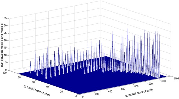
Fig. 7Distribution of Was2 between cylindrical shell modes and its cavity modes with same m and n
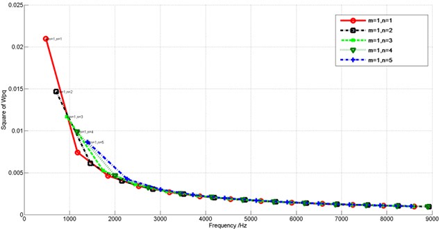
Fig. 8Radiation efficiency of simply-supported cylindrical shell
4.1. Validation case
Figure 9 shows a cylindrical shell coupled to its cavity (with parameters in Table 1) for validation case. The shell is divided into 9072 quadrangle elements and the cavity is divided into 61236 hexahedral elements. Figure 10 compares the radiation efficiencies obtained analytically (as in Sec. 3.2) and numerically (with FEM results). As it can be seen, the results agree well when the frequency is over 1600 Hz, although the numerical method slightly overestimates the radiation efficiencies at 1000 Hz and 1250 Hz. The discrepancy is due to a slight overestimation of modal works on the coupling surface during numerical interpolation. Overall, the accuracy shown by the integrated FEM-SmEdA is acceptable.
4.2. Radiation efficiency of a conical shell
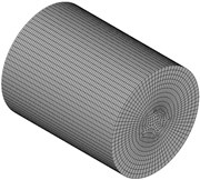
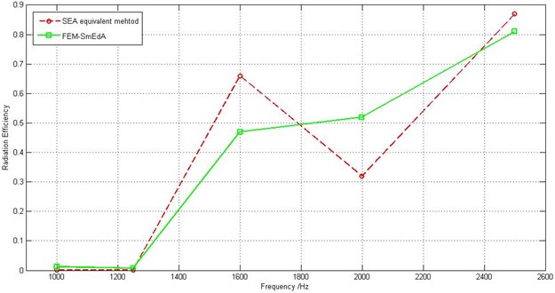
Truncated cone is a typical geometry of stressed-skin structures in aerospace engineering. In classic SEA, a conical shell is usually simplified to a cylindrical shell with the same conic length and surface area to obtain its radiation efficiency, and thus obvious errors will occur in this treatment. Figure 11 shows a typical conical shell model, and Table 5 tabulates the corresponding parameters. Figure 12 compares the radiation efficiencies obtained by the proposed FEM-SmEdA algorithm and the SEA equivalent approach. As it can be seen, there is an obvious difference between the two results. The difference between the two methods demonstrates that the traditional SEA equivalent method produces large errors and could be replaced by the present FEM-SmEdA approach.
Table 5Cavity and conical shell characteristics
Cavity | Cylindrical shell | ||
(m) | 0.113 | (m) | 0.113 |
(m) | 0.4 | (m) | 0.4 |
(m) | 1 | (m) | 1 |
(kg/m3) | 1.2 | (m) | 0.004 |
(m/s) | 340 | (kg/m3) | 7820 |
0.01 | (Pa) | 2.1e11 | |
0.3 | |||
0.01 | |||
Fig. 9FEM meshes of validation case
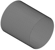
a) Mesh of the cylindrical shell
b) Mesh of the cavity
Fig. 10Comparison between analytical and FEM results
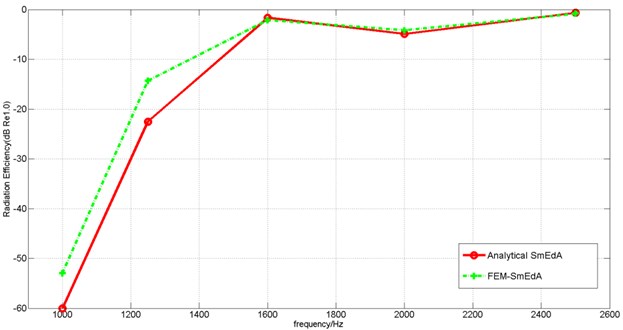
Fig. 11Geometry of a conical shell
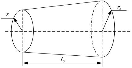
Fig. 12Comparison between FEM-SmEdA and SEA equivalent results
5. Conclusions
In this paper, an integrated FEM-SmEdA algorithm is proposed for the calculation of radiation efficiency for shell structures to their cavities. The radiation efficiencies of cylindrical and conical shells were investigated and compared in detail by different approaches. In cylindrical shell case, analytical SmEdA provides closer results to the experimental one than the conventional wave method and SEA approach, especially in low frequency band, which is due to the better representation of boundary conditions. Furthermore, the validity of the proposed FEM-SmEdA algorithm is demonstrated by a comparison study with the theoretical SmEdA approach. In conical shell case, the integrated FEM-SmEdA algorithm was applied in comparison with the conventional SEA approach. The discrepancy between the two approaches indicates that the conventional SEA algorithm should be taken place by the proposed one to obtain more accurate results in practical engineering analysis.
References
-
Maidanik G. Response of ribbed panels to reverberant acoustic fields. Journal of Acoustical Society of America, Vol. 34, Issue 6, 1962, p. 809-826.
-
Wallace C. E. Radiation resistance of a rectangular panel. Journal of Acoustical Society of America, Vol. 51, Issue 3, 1972, p. 946-952.
-
Xie G., Thompson D. J., Jones C. J. C. The radiation efficiency of baffled plates and strips. Journal of Sound and Vibration, Vol. 280, Issue 1-2, 2005, p. 181-209.
-
Ren H. J., Sheng M. P. A thin rectangular plate's modal radiation efficiency. Mechanical Science and Technology for Aerospace Engineering, Vol. 29, Issue 10, 2010, p. 1397-1400.
-
Snyder S. D., Tanaka N. Calculating total acoustic power output using modal radiation efficiencies. Journal of Acoustical Society of America, Vol. 97, Issue 3, 1995, p. 1702-1709.
-
Putra A., Thompson D. J. Sound radiation from rectangular baffled and unbaffled plates. Applied Acoustics, Vol. 71, Issue 12, 2010, p. 1113-1125.
-
Manning J. E., Maidanik G. Radiation properties of cylindrical shells. Journal of Acoustical Society of America, Vol. 36, Issue 9, 1964, p. 1691-1698.
-
Szechenyi E. Modal densities and radiation efficiencies of unstiffened cylinders using statistical methods. Journal of Sound and Vibration, Vol. 19, Issue 1, 1971, p. 65-81.
-
Ramachandran P., Narayanan S. Evaluation of modal density, radiation efficiency and acoustic response of longitudinally stiffened cylindrical shell. Journal of Sound and Vibration, Vol. 304, Issue 1-2, 2007, p. 154-174.
-
Cheng Z., Fan J. Radiation efficiency of submerged finite stiffened cylindrical shell. Journal of Ship Mechanics, Vol. 16, Issue 10, 2012, p. 1218-1228.
-
Wang C., Lai J. C. S. The sound radiation efficiency of finite length acoustically thick circular cylindrical shells under mechanical excitation I: Theoretical analysis. Journal of Sound and Vibration, Vol. 232, Issue 2, 2000, p. 431-447.
-
Wang C., Lai J. C. S. Acoustic radiation of finite length cylindrical shells with different boundary conditions using boundary element method. Proceedings of 5th International Congress on Sound and Vibration, Vol. 2, 1997, p. 877-884.
-
Maxit L., Guyader J. L. Estimation of SEA coupling loss factors using a dual formulation and FEM modal information, Part I: Theory. Journal of Sound and Vibration, Vol. 239, Issue 5, 2001, p. 907-930.
-
Maxit L., Guyader J. L. Estimation of SEA coupling loss factors using a dual formulation and FEM modal information, Part II: Numerical applications. Journal of Sound and Vibration, Vol. 239, Issue 5, 2001, p. 931-948.
-
Totaro N., Dodard C. SEA coupling loss factors of complex vibro-acoustic systems. Journal of Vibration and Acoustics, Vol. 131, Issue 4, 2009, p. 1-8.
-
Lyon R. H., De Jong R. G. Theory and Application of Statistical Energy Analysis. Second Edition, MIT Press, Cambridge, MA, 1998.
-
Cremer L., Heckl M., Petersson B. A. T. Structure-Borne Sound. Third Edition, Springer-Verlag, Berlin, 1998.
About this article

