Abstract
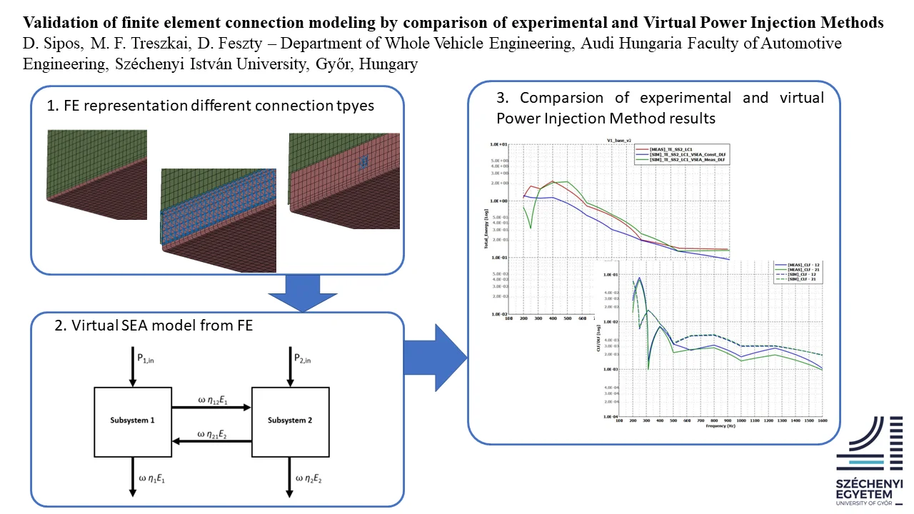
There are several ways to obtain the matrix of damping loss factors and coupling loss factors for Statistical Energy Analysis. The most recent approach is Virtual SEA, where the Power Injection Method is performed virtually on a finite element model. In order to validate this approach, the most common connection types are investigated in this paper through an L-junction of two coupled steel plates. Virtual SEA and experimental Power Injection Method results are compared in a bent, line welded, superglued and spotwelded variants. The respective finite element connection representation is also validated during the comparison. It was found that with the correct simulation setup, Virtual SEA provides good agreement with the experimental results. In case of the spotwelded variants, further investigations were necessary regarding the parameters of the connection. The influence of these parameters was evaluated and the greatest source of deviations in the results is found.
Highlights
- Experimental and virtual Power Injection Methods are compared
- Different FE connection types are investigated through Virtual SEA
- Effects of FE connection parameters on the Virtual SEA CLFs are explored
1. Introduction
For a wide range of industrial applications, the role of Computer-Aided Engineering (CAE) tools is increasing in order to predict the characteristics of the products via simulations. This trend is valid for the vibroacoustic analysis of vehicles too. Vehicle manufacturers put huge efforts in the Noise, Vibration and Harshness (NVH) developments of their products, since the vibrational comfort and the acoustics of the vehicle became one of the most important factors of customer satisfaction.
There are several well-established CAE methods available for NVH development, such as Finite Element Method (FEM) or the Statistical Energy Analysis (SEA) methods, which application is typically driven by the frequency range to be captured. FEM is more suitable for low-frequency problems and can be used for detailed modeling of the structure. As the frequency goes higher, the required element size decreases, resulting in a large number of elements. The consequence of the fine mesh are the drastically increased computational costs. SEA on the other, deals with high frequency problems with negligible computational costs, using spatial averaging and power balance equations. The drawbacks of this method are that due to its very nature, it does not allow detailed modeling of the structure as well as that the coefficients that drive the power balance equations are very challenging to obtain. These coefficients are the Damping Loss Factors (DLF) and the Coupling Loss Factors (CLF) that represents the dissipated and the exchanged power in the system. Various approaches are available to obtain them, such as analytical SEA [1-3]; experimental SEA (also called as Power Injection Method-PIM) [4-7]; and Virtual SEA [8-9]. The latter attempts to put the PIM into the virtual environment using FEM, thus eliminating the necessity of conducting experiments. Each of these approaches will be overviewed shortly in the next chapters.
Several papers deal with the analytical and experimental determination of CLFs and DLFs for coupled plates. Treszkai et al. [10] investigated 19 different joining methods and compared experimental results to analytical SEA results. Panuszka et al. [11] investigated L-shaped structures with different joint types and thickness ratios. They estimated the DLFs from reverberation time, the CLFs from the power balance equation and compared the results to analytical formulas. Le Bot and Cotoni [12] investigated the validity of coupled plates SEA model through direct numerical simulations. Patil and Manik [13] performed a sensitivity analysis of differently coupled plates using direct differentiation and finite difference methods. However, these studies do not provide validation for coupled plates in Virtual SEA.
Therefore, the goal of present study is to evaluate the results of the experimentally and the virtually performed power injection method in different coupling conditions. This will be carried out by comparing the measured and calculated coupling loss factors and by comparing the energy responses to a given injected power. To do so, the least possible complex test cases were assembled, also described in the next chapters. The experimental data was provided by former measurements, carried out in the work of Treszkai et al. [10]. The finite element modeling method of each connection type can be also validated through this comparison. In each case, the virtual PIM was performed in MSC Actran’s Virtual SEA module, for which, the modal extraction was done in MSC Nastran.
2. Statistical energy analysis
Statistical Energy Analysis is an energy-based approach for describing the vibro-acoustic behavior of complex structures, introduced by Lyon and Maidanik [14] and Smith [15] in the 1960s. It is suitable for high-frequency analyses, where the response of the structure can only be described by statistical methods. It assumes that certain conditions are fulfilled, such as the weak coupling, the homogenous vibrational energy distribution in subsystems and sufficient modal density. The SEA power balance equation can be written for subsystem as [16-17]:
where equals the total injected power, is the exchanged power between subsystem and . is the dissipated power from subsystem given by [17]:
where is the damping loss factor, is the center frequency of the considered frequency band, is the subsystem energy. The power exchanged is assumed to be [17]:
where and are the coupling loss factors. The general form of the power balance equation for any number of subsystems can be written as [17]:
or in compact form [17]:
Fig. 1 shows an SEA power balance model for 2 subsystems, which is the schematic representation of the test cases that this paper investigates.
Fig. 1Schematic representation of the SEA power balance model [10]
![Schematic representation of the SEA power balance model [10]](https://static-01.extrica.com/articles/22754/22754-img1.jpg)
As said, the most challenging part of an SEA study is to obtain the loss matrix , containing all of the coupling and damping loss factors. There are several different approaches to consider. The first method is the analytical SEA method. As the name suggest, it uses analytical formulations to estimate the coupling conditions between any two neighboring subsystems inferred by the transmission coefficient of the junction. This means that the analytical formulation for the Coupling Loss Factors (CLF) can only be derived for physically connected subsystems for which, these formulas are available e.g., simple connections for regular geometrical objects. Indirect coupling loss factors that are often associated with global modes cannot be considered. However, as opposed to the experimental SEA that will be described in the next chapter, analytical SEA considers energy exchanges associated with all wave types [17].
3. Power injection method
The SEA loss matrix can also be obtained by experimental measurements. In the Power Injection Method, which was first introduced by De Langhe [4], the loss matrix is calculated by substituting the and values in the SEA power balance equation. The most convenient way to do so is to excite all subsystems one by one while measuring the injected power and the response of all the other subsystems. There are various descriptions of the mathematical background of this theory, however, the one below is largely based on Ref. [17]. According to this, the injected power to a subsystem can be calculated according to the following equation:
where is the excitation force and is the driving point mobility. The kinetic energy of the subsystem is given by:
where is the mass, and denotes the spatially averaged squared vibrational velocity of the subsystem. After iterating on all subsystems, on the left-hand side of the SEA power balance equation, a diagonal matrix and on the right-hand side, a full matrix of is produced as shown by Eq. (8):
From the above equation, the loss matrix can be obtained by a simple matrix inversion. It should be noted that this method considers energy exchanges associated with only bending waves and not with longitudinal or shear waves. It is also a drawback of this method that it needs access to a prototype to perform the measurements on and it can require extreme amounts of measurements and man hours depending on the size of the structure.
The most recent approach to obtain the SEA loss matrix is the Virtual SEA method, first introduced by Gagliardini et al. [8]. They used finite element calculations to build up an energy distribution model for the virtual power injection method. Based on the modal representation of the vibro-acoustic model, the distribution matrices enable the computation of energetic quantities on element patch levels i.e., k set of elements. Considering an element patch , the associated mass and stiffness distribution matrices are obtained by projecting the set of element level mass and stiffness matrices on the modal basis :
A generic kinematic quantity expressed in modal coordinates as: . Since energetic quantities generally takes the expression , it can be rewritten as where is either the mass or stiffness distribution matrix of element patch . Thus, the distribution matrices can be directly used to calculate energetic quantities. Without further derivation, the injected power can be expressed as:
The potential and kinetic energies expressed as:
And the dissipated power is given by:
Once the energy distribution model is built up, it can be used for the power injection method, meaning exciting each subsystem one by one, while monitoring the response in all the other subsystems, exactly as in experimental SEA. However, this method combines the advantages of the previously mentioned approaches, but without their limitations and challenges: all of the wave types can be considered, no difficulties caused by measurements and any complex geometries can be assessed. The so obtained coupling matrix should approximate the SEA assumptions as close as possible and it only requires a finite element modal analysis to be available. In the next chapter, these finite element models will be reviewed, each with different connection type in order to validate the modeling methods and the virtually performed PIM.
4. Test cases and simulation models for loss matrix estimation
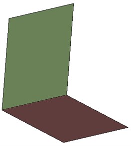
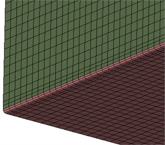
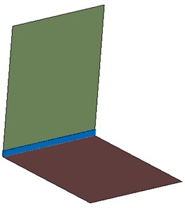
Some of the most common connection types were investigated in this study, based on the work of Treszkai et al. [10] The first model was a single piece of sheet metal bent in 90° with 2 mm nominal thickness. The junction created by the bending split the structure into 2 subsystems. Plate 1 will be excited along all the load cases and will be referenced as subsystem 1 and Plate 2 will be the receiver, named subsystem 2. The dimensions of the plates are approximately 650×550 mm, but due to the connection to be realized, there is a 20 mm overlapping area between the plates. This overlap for the connection was always formed from Plate 1 and bent in 90°, as described in [10]. The finite element model of the bent variant is shown in Fig. 2.
Fig. 2Finite element model of test Case 1: the baseline bent variant
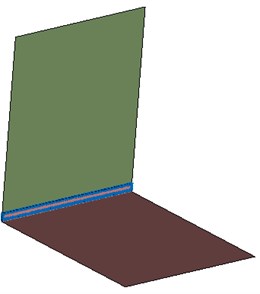
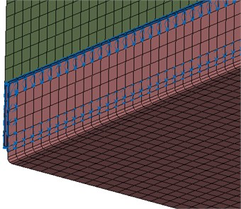
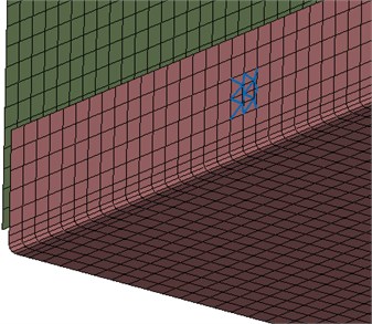
In the second variant, the two plates were connected with line welding as shown by the representative finite element model in Fig. 3. The elements used for the realizing the connections are NASTRAN-specific, each of those description can be found in the corresponding documentations. The line welding was modeled as RBE3-HEXA-RBE3 connection with one row and one layer of HEXA elements. The material properties of the solid elements were the same as the plates. The line welding connection was created around the overlapping area just as on the physical model.
Fig. 3Finite element model of test Case 2: the line welded variant
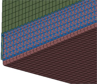
In the third variant, a superglued type of connection was created. The whole overlapping areas on both plates were connected, again with RBE3-HEXA-RBE3 elements shown by Fig. 4. The gap between the plates was filled with 3 layers of HEXA elements and those material properties were set according to Table 1:
Table 1Material properties of the superglue
Young’s modulus | 1630 MPa |
Poisson ratio | 0.45 |
Density | 1200 kg/m3 |
Fig. 4Finite element model of test Case 3: the superglued variant.
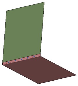
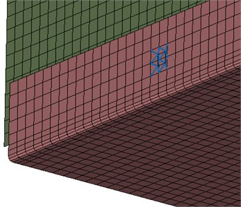
The last variant that is covered here was the spotwelded connection. 5 connection points were equally spaced in the overlapping area, as shown by Fig. 5. The finite element representation of this type of connection is again RBE3-HEXA-RBE3. This time, a single HEXA element was created in the connection and similarly to the line welded variant, the material properties of the solid elements were set to steel.
Fig. 5Finite element model of test Case 4: the spotwelded variant
The measurement process that provided the data for this comparison is described more in detail in [10]. In short, impact testing methodology was employed with a total of 12 accelerometers per plates in 4 runs. The injected power was measured according to Eq. (6) and the responses were calculated according to Eq. (7). Free-free boundary condition was ensured during the measurements.
Regarding the finite element simulation models, the maximum element size was 5 mm, which enables the models to be valid above the frequency of interest. The modal bases were calculated up to 2000 Hz for building up the energy distribution models. The SEA subsystem division was also kept the same during the analyses. The finite elements created for the connections were always assigned to the receiver plate’s subsystem. For each variant, two Virtual SEA simulations were set up. One with constant damping, that assumes no measurements had been made in prior the simulations and one where the damping values of the plates are exactly matching the measured DLF values. The constant damping value of the plates was set according to 0.2 %, which is a typical value for such lightly damped steel plates. Both Virtual SEA variants were excited with the exact same injected power that comes from the measurements to make the results the as comparable as possible.
The results that will be investigated are the energy levels of the receiver plate, subsystem 2. Measured curves will be compared to simulation results, one with constant damping loss factors and one with measured damping loss factors. The second type of comparison for each variant investigates the comparison of coupling loss factors. In this case, since the damping and coupling loss factors are dependent on each other, the measured curves will only be compared to the simulation where the measured damping loss factors were employed. Thereby, no external factors affect the result, so one can get a more accurate insight to the differences of the measured and the calculated coupling loss factors by the Virtual SEA method. It should be noted that the measured coupling loss factors are quite challenging to capture accurately. Moreover, if the SEA weak coupling condition is assured, large discrepancies can occur in the coupling loss factors whose effects may not appear in the energetic results of the receiver plate.
5. Results and analyses
5.1. Test Case 1: baseline bent variant
Fig. 6 shows the energy response of the receiver plate in measurement and Virtual SEA simulations. It can be observed that the 0.2% constant damping value employed in the simulation (blue curve) still might be too high, proven by the measured values as well, which were lower in general. The simulation employing the exact damping values (green curve) agrees very well with the measurement. The general trend of both the results is still acceptable and both curves reflect the real behavior of the structure.
The comparison of the measured and calculated coupling loss factors is shown by Fig. 7. It can be observed that in the measurement and in the simulation too, the reciprocity relation is respected. In the low frequency range, larger discrepancies can occur but as the frequency increases, the results get more accurate. Starting from about 300 Hz, the trends are relatively well captured, except in the 1000 Hz third octave band. This effect is slightly visible in the energy response curves as well. Overall, the bent model has few parameters to tune, thus this level of correlation is expected. The discrepancies can be attributable to the high sensitivity of the model.
Fig. 6Energy response of the receiver plate for Test Case 1: baseline bent variant. Measurement – red curve; simulation with constant damping – blue curve; simulation with measured damping – green curve
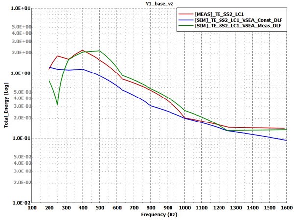
Fig. 7Coupling loss factors for test Case 1: baseline bent variant. Measurement – solid lines; simulation – dashed lines
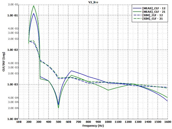
5.2. Test Case 2: line welded variant
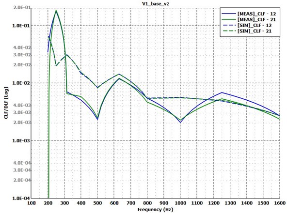
The energy response of plate 2 in the line welded variant is shown by Fig. 8. This time both simulation curves are in good agreement with the measurement. The 0.2 % constant damping value for this variant seems to be appropriate (blue curve). The simulation with the measured damping value (green curve) has discrepancies in certain third octave bands in the low frequency range and in the 500 Hz band. These bands have the largest difference in terms of coupling loss factors too, as Fig. 9 suggests. Despite this, the rest of the results in this frequency range is in good agreement with the measurement and overall, for such sensitive structure, thus the modelling method for line welding can be approved.
Fig. 8Energy response of the receiver plate for Test Case 2: line welded variant. Measurement – red curve; simulation with constant damping – blue curve; simulation with measured damping – green curve
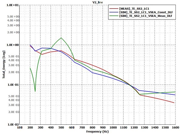
Fig. 9Coupling loss factors for test Case 2: line welded variant. Measurement – solid lines; simulation – dashed lines
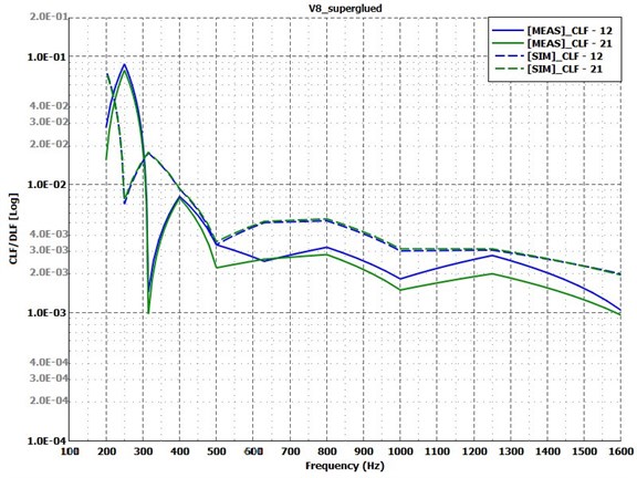
5.3. Test Case 3: superglued variant
The next variant to compare the results of is the superglued one. Fig. 10 shows, with the approximated constant damping (blue curve), the simulation model is a little bit overdamped below 600 Hz but above that frequency, it gives reliable results. The simulation model with the measured damping (green curve) is almost perfectly catches the measurement curve in every third octave frequency bands. Fig. 11 shows the comparison of the measured and calculated CLFs. It can be observed that the nature of these curves is well represented by the Virtual SEA simulation from 400 Hz, though the amplitudes are not necessarily correct. However, this does not have a great impact on the energy response curves, as it could be seen on Fig. 10.
Fig. 10Energy response of the receiver plate for Test Case 3: superglued variant. Measurement – red curve; simulation with constant damping – blue curve; simulation with measured damping – green curve
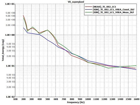
Fig. 11Coupling loss factors for test Case 3: superglued variant. Measurement – solid lines; simulation – dashed lines
5.4. Test Case 4: spotwelded variant
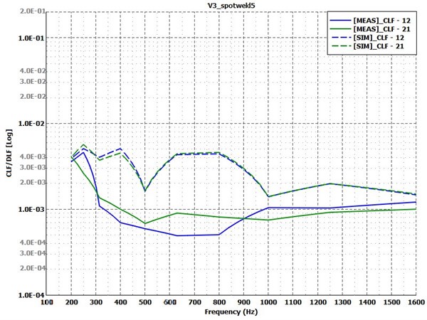
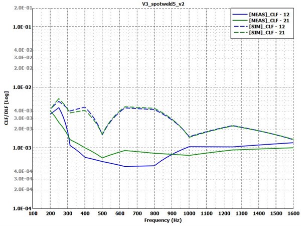
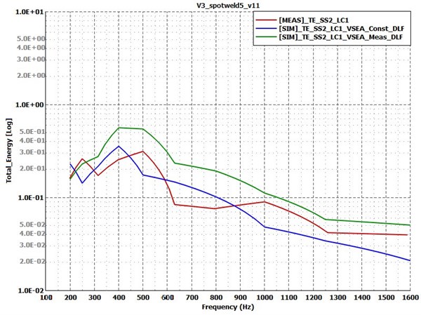
Last, the results of the spotwelded variants are compared on Fig. 12 and Fig. 13. Former shows that the energy response of the receiver plate has the largest difference between simulation and measurement along all of the variants. The simulation with the measured damping values (green curve) shows similarities with the experimental results in terms of trends, but far from the exact values. The constant damping value for this variant does not provide reliable results in this form. Regarding the measured and calculated coupling loss factors shown by Fig. 13, it is obvious that something is wrong with either the modelling method of the spotwelded connection or with the measurement. To find out what could cause such differences, a few more simulation model variants were derived, and the effect of each parameter was investigated in the same way.
Fig. 12Energy response of the receiver plate for Test Case 4: spotwelded variant. Measurement – red curve; simulation with constant damping – blue curve; simulation with measured damping – green curve
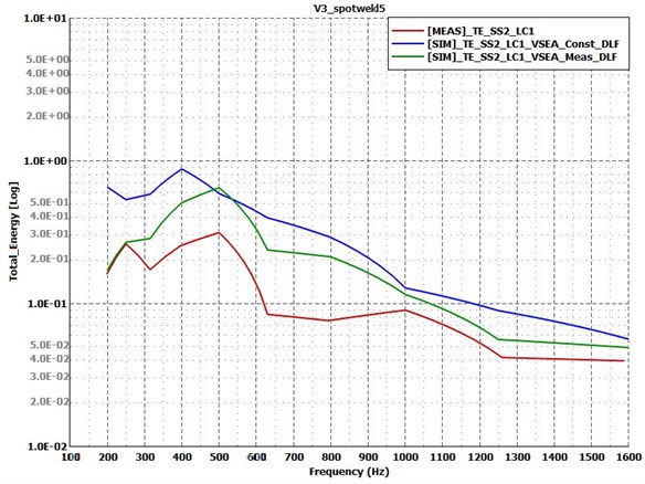
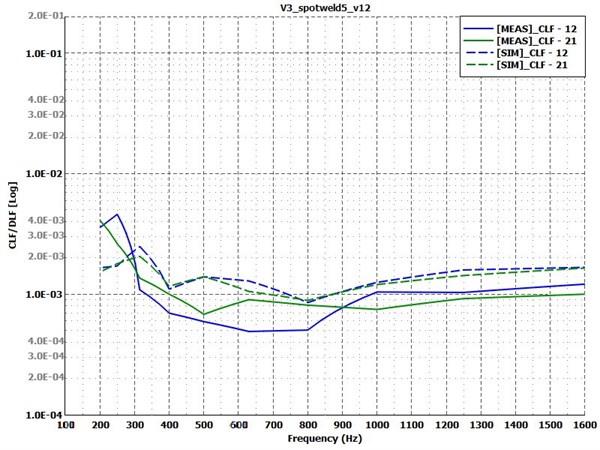
Fig. 13Coupling loss factors for test Case 4: spotwelded variant. Measurement – solid lines; simulation – dashed lines
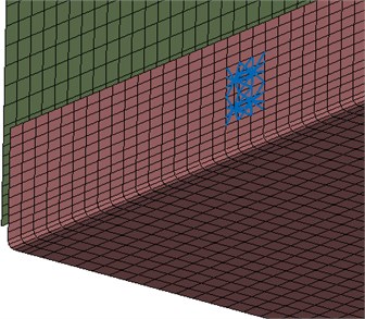
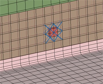
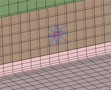
The first parameter that was changed concerns the RBE3-HEXA-RBE3 connection. The radius of the connecting region was increased by approximately a factor of 2 via involving more grids in the RBE3 element, shown by Fig. 14. Fig. 15 and Fig. 16 show the so-obtained results. These curves suggest that the radius of the spotweld connection has minor influence on both the energetic response and the coupling loss factors in this case. Therefore, it is unlikely that this parameter is responsible for the large discrepancies in the results on its own.
Fig. 14Increased RBE3 diameter and connecting region in Test Case 4: spotwelded variant. a) – original model; b) – increased RBE3 diameter
a)
b)
In the next step of the investigation, several changes were made to the model. As Fig. 17 shows, the size of the HEXA element in the connection was reduced from 5 mm to about 2 mm. In order to soften the connection, the Young’s modulus of it was also changed from 210000 MPa to 100000 MPa. Since the simulation results with the constant damping values were too underdamped, the global structural damping value was increased from 0.2 % to 0.5 %. In the simulation with the measured damping values, the damping of the plates was unchanged. However, the damping of the HEXA elements is defined individually and was increased from 0.2 % to 1 %, because this model also seemed to be underdamped.
Fig. 15Energy response of the receiver plate for Test Case 4: spotwelded variant with increased connection area. Measurement – red curve; simulation with constant damping – blue curve; simulation with measured damping – green curve
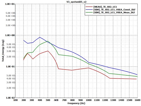
Fig. 16Coupling loss factors for test Case 4: spotwelded variant with increased connection area. Measurement – solid lines; simulation – dashed lines
The combined effect of these changes is shown by Fig. 18 and Fig. 19. Regarding the simulation results with the unchanged plate damping values with the green curve, all of these changes had once again just minor effect, compared to previously seen curves on Fig. 15 and Fig. 16. Only slight improvements were achieved. It is conspicuous though that the increase in the constant damping in case of the blue curve does have significant effect on the order of magnitude of the receiver plate’s response, but now it seems to be overdamped, compared to the measured curve. However, the comparison of coupling loss factors suggests that neither of these changes improved the overall quality of the model, hence they cannot be stated as valid.
Fig. 17Reduced HEXA element size in comparison for Test Case 4: spotwelded variant: a) – original model; b) – reduced HEXA element
a)
b)
Fig. 18Energy response of the receiver plate for test Case 4: spotwelded variant with increased damping, decreased connection stiffness. Measurement – red curve; simulation with constant damping – blue curve; simulation with measured damping – green curve
The effect of each of the above-mentioned parameters was also investigated separately in order to make sure that opposite effects do not take place and extinguish each other out, but that was not the case. Only the increased constant damping had large influence on its own, but as it was seen on Fig. 18 and Fig. 19, the offset of the response curve does not mean a substantial improvement in quality.
Many of the presumed influencing factors of the finite element connection modelling method were investigated with no success in terms of the representation of the measured curves. In the next step, it was assumed that the physical model had deviations from the nominal dimensions. Thus, each of the plates’ thicknesses were increased from 2 mm to 2.1 mm in the simulation models and the increased damping values were also kept. This produced similar results as seen on Fig. 18 and Fig. 19. In the next step, the ratio of the thicknesses was changed, so only Plate 1 was increased to 2.1 mm. Fig. 20 and Fig. 21 show that this improved further the energy response on the receiver plate compared to the previously seen changes, regarding the green curve with the measured damping values applied on both plates. The constant damping simulation curve is also changed, and its trend seems to be better fitting the experiment and the simulation with the exact damping values, but it is still overdamped. More fine tuning of the global damping value will be needed to this model in order to get better results, but as the green curve suggests, the model itself became more accurate. The point is, that significant improvement was achieved in terms of the coupling loss factors. The trend of these curves is now fairly well captured, which was not the case with the previous models at all. Of the many coupling parameters that were tested, the ratio of the thicknesses had real effect on the simulation results, and it provided the only way to really approach the measured curves. The connection modelling method in this case can now be assumed to be correct.
Fig. 19Coupling loss factors for test Case 4: spotwelded variant with increased damping, decreased connection stiffness. Measurement – solid lines; simulation – dashed lines
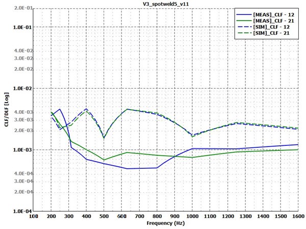
Fig. 20Energy response of the receiver plate for test Case 4: spotwelded variant with different thickness ratio. Measurement – red curve; simulation with constant damping – blue curve; simulation with measured damping – green curve
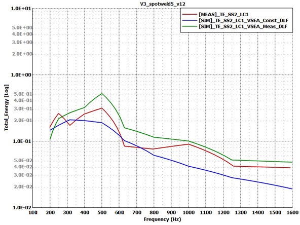
Fig. 21Coupling loss factors for test Case 4: spotwelded variant with different thickness ratio. Measurement – solid lines; simulation – dashed lines
6. Conclusions
In this study, the finite element modelling method of some of the most common connection types was investigated through comparison of experimental and virtual power injection method. These connection types were: 1) bent; 2) line welded; 3) superglued; 4) spotwelded. Two type of simulation results were tested to measurement data in each case: first, based on no experimental data, where the global damping of the simulation model was a constant value; and second, where the damping of the two plates came from the experimental PIM to get a better understanding of the behavior of the other influencing factors and a better insight to the validity of the models. In case of the bent, line welded and superglued variants, the simulation models reflected the realistic behavior of the physical models, apart from some low frequency discrepancies where probably the SEA assumptions were not entirely respected. The overall quality of these models was satisfactory, in terms of the response of the receiver plate and the coupling loss factors too. However, the spotwelded variant showed unexpectedly large differences. The effect of the main influencing factors of the connection modeling method was investigated. It was found that the changes made to the involved area in the connection, the stiffness, damping and dimensions of the connecting elements all had relatively small effect on the resulting response and coupling loss factor curves. The increase in the global damping value had large influence on the energy response as expected, but it does not account for the different behavior of the model. The only thing that brough the simulation results closer to the measurement was the change in the thickness ratio of the two plates. Assuming that Plate 1’s thickness differed from the nominal 2 mm nominal value to 2.1 mm, the simulation curves improved significantly. It was proved that the connection modeling method used for spotwelded connection can be regarded valid once the exact dimensions of the models are clarified. Further studies may investigate in the same manner the other connection types that had been studied in [10], e.g., the bolted type, the more densely spotwelded one or all of those variants in a different connection angle. These would provide valuable results on validity of the finite element modeling of each connection type.
References
-
S. Preis and G. Borello, “Prediction of light rail vehicle noise in running condition using SEA,” in INTER-NOISE and NOISE-CON Congress and Conference Proceedings, 2016.
-
H. A. Dande, T. Wang, J. Maxon, and J. Bouriez, “SEA model development for cabin noise prediction of a large commercial business jet,” Noise and Vibration Conference and Exhibition, Jun. 2017, https://doi.org/10.4271/2017-01-1764
-
P. Tathavadekar, R. O. de Alba Alvarez, M. Sanderson, and R. Hadjit, “Hybrid FEA-SEA modeling approach for vehicle transfer function,” in SAE 2015 Noise and Vibration Conference and Exhibition, Jun. 2015, https://doi.org/10.4271/2015-01-2236
-
K. de Langhe, “High frequency vibrations: contributions to experimental and computational SEA parameter identification techniques,” Ph.D. Thesis, KU Leuven, 1996.
-
M. Bouhaj, O. Von Estorff, and A. Peiffer, “An approach for the assessment of the statistical aspects of the SEA coupling loss factors and the vibrational energy transmission in complex aircraft structures: Experimental investigation and methods benchmark,” Journal of Sound and Vibration, Vol. 403, pp. 152–172, Sep. 2017, https://doi.org/10.1016/j.jsv.2017.05.028
-
P. P. James and F. J. Fahy, “A technique for the assessment of strength of coupling between sea subsystems: experiments with two coupled plates and two coupled rooms,” Journal of Sound and Vibration, Vol. 203, No. 2, pp. 265–282, Jun. 1997, https://doi.org/10.1006/jsvi.1996.0871
-
D. A. Bies and S. Hamid, “In situ determination of loss and coupling loss factors by the power injection method,” Journal of Sound and Vibration, Vol. 70, No. 2, pp. 187–204, May 1980, https://doi.org/10.1016/0022-460x(80)90595-7
-
L. Gagliardini, L. Houillon, L. Petrinelli, and G. Borello, “Virtual SEA: mid-frequency structure-borne noise modeling based on finite element analysis,” in SAE 2003 Noise and Vibration Conference and Exhibition, May 2003, https://doi.org/10.4271/2003-01-1555
-
D. Sipos, M. Brandstetter, A. Guellec, J. Jacqmot, and D. Feszty, “Extended solution of a trimmed vehicle finite element model in the mid-frequency range,” in 11th International Styrian Noise, Vibration and Harshness Congress: The European Automotive Noise Conference, Sep. 2020, https://doi.org/10.4271/2020-01-1549
-
M. F. Treszkai, A. Peiffer, and D. Feszty, “Power injection method-based evaluation of the effect of binding technique on the coupling loss factors and damping loss factors in statistical energy analysis simulations,” Manufacturing Technology, Vol. 21, No. 4, pp. 544–558, Sep. 2021, https://doi.org/10.21062/mft.2021.065
-
R. Panuszka, J. Wiciak, and M. Iwaniec, “Experimental assessment of coupling loss factors of thin rectangular plates,” Archives of Acoustics, Vol. Vol. 30, No. 4, pp. 533–551, 2005.
-
A. Le Bot and V. Cotoni, “Validity diagrams of statistical energy analysis,” Journal of Sound and Vibration, Vol. 329, No. 2, pp. 221–235, Jan. 2010, https://doi.org/10.1016/j.jsv.2009.09.008
-
V. H. Patil and D. N. Manik, “Sensitivity analysis of a two-plate coupled system in the statistical energy analysis (SEA) framework,” Structural and Multidisciplinary Optimization, Vol. 59, No. 1, pp. 201–228, Jan. 2019, https://doi.org/10.1007/s00158-018-2061-9
-
R. H. Lyon and G. Maidanik, “Power flow between linearly coupled oscillators,” The Journal of the Acoustical Society of America, Vol. 34, No. 5, pp. 623–639, May 1962, https://doi.org/10.1121/1.1918177
-
P. W. Smith, “Response and radiation of structural modes excited by sound,” The Journal of the Acoustical Society of America, Vol. 34, No. 5, pp. 640–647, May 1962, https://doi.org/10.1121/1.1918178
-
Shorted, P., Cotoni, and V., Statistical Energy Analysis in Engineering Vibroacoustic Analysis: Methods and Applications. United Kingdom: John Wiley and Sons, 2016.
-
“Actran 2022 User’s guide Vol. 1: Installation, Operations, Theory and Utilities,” Free Field Technologies, 2022.
About this article

This work is supported by the Hungarian Academy of Sciences and Audi Hungaria Zrt. through the funding provided to the MTA-SZE Lendület Vehicle Acoustics Research Group.
The datasets generated during and/or analyzed during the current study are available from the corresponding author on reasonable request.
The authors declare that they have no conflict of interest.
