Abstract
The recent increase in the use of the railway and the establishment of more restrictive policies of harmful environmental effects of railway transport highlights the need to investigate ground vibrations related to trains. Therefore models to evaluate how this phenomenon affects have been performed. This article aims to expose both analytical and 3D-FE models and to compare theoretical formulation and results. Models have been calibrated and validated with real data. Furthermore, a simulation of the acceleration level of different railway infrastructure elements has been achieved.
1. Introduction
Railway transport networks have been growing over centuries as a consequence of continuous increase of volumes of passengers and goods. The ground vibrations induced by traffic can propagate through the surrounding soils to adjacent buildings, causing annoyance to residents or affecting delicate instruments located inside. More than 12 million EU inhabitants are affected by railway vibration during the day and 9 million during the night. In last years EU regulations on railway vibration and noise have been: arise emission limits and achieve a harmonised measurement method.
The current social and technological development is bringing about increasingly stringent requirements of environmental conditions, both in terms of safety and comfort. The vibrations generated by the passage of trains around which in the past might seem tolerable, today are considered as major annoyances. The traffic induced vibrations are one of the most important, second only are generated vibrations in industrial environments or areas of execution of works.
Under these premises, the interest in studying and modelling ground vibrations caused by railway traffic has been increased in recent years. To carry out this undertaking, analytical and numerical models have been developed during the last decades.
This paper presents a main objective: the theoretical and experimental comparison of results obtained by analytical and numerical models of railway vibrations previously developed in [1] and [2] respectively. Furthermore, it is pretended to simulate by analytical and numerical models the accelerogram of different infrastructure elements. Both models have been calibrated and validated with real data gathered on Santander-Liérganes line, in the north of Spain. This line is operated by FEVE (Ferrocarriles Españoles de Vía Estrecha).
The origin of railway vibration modelling started in 70s. First of all, dissipation mechanisms of vibrations were presented in [2] and [3]. In [4] an analytical study of the vibrations induced in tunnel metropolitan structures was developed. Reference [5] continued in this way, in order to perform an accurate model taking into account generation, transmission and reception subsystems, which contribute in the global vibration phenomenon. Later more analytical models have been generated. Reference [6] presented an important improvement in the way loads, dividing loads into quasi-static and dynamic forces. References [7] and [8] continued in the development of the model proposed by [6], and form the basis of the analytical model completed in [1].
With the advances of computational resources, different numerical models of railway ground vibrations have been emerging. Finite Element Method (FEM) has been one of the most employed for numerical modelling to predict vibration levels caused by railway traffic. In [9] the dynamic response of an embedded rail track was determined using FEM. Later [10] studied how propagation of waves was mitigated by buried walls through 2D FEM.
2. Brief description of railway section and acceleration data collection
Section of study is located in a straight track stretch of the Santander-Lierganes line in Cantabria, Spain. As it has been said, the operator of the line is FEVE and consists on a conventional ballasted track with UIC 45 rails and wooden sleepers. The track gauge is 1 meter. The line is transited by vehicles CAF S/3800, formed by three carriages and six bogies. Mean speed of trains when data were gathered was 25 km/h.
For data collection three Sequoia FastTracer® triaxial accelerometers based on MEMS technology were used to measure accelerations on the track. Sensors characteristics and location are explained in [1].
3. Analytical model
The analytical model presented in this paper has been previously developed in [1]. This formulation follows the same theories presented in [11] and [12].
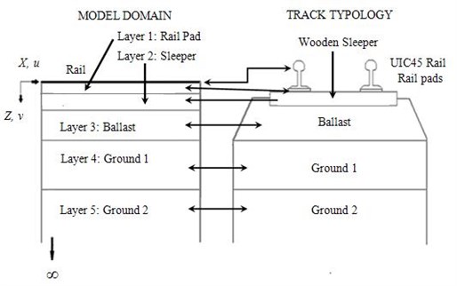
The model is capable to predict vertical displacements and stresses induced by dynamic and quasi-static loads in the depth () direction. In order to achieve these values, railway section was modeled in 2D in the track axis plane. Railway infrastructure was defined by five layers, each one representing the different infrastructure elements (rail pad, sleeper, ballast, ground 1 and ground 2) (see Fig. 1). At the top of the section a Timoshenko beam models rail behavior.
Fig. 1Model scheme
Model core equation is the wave equation expressed in vectorial terms:
where is the displacement vector , and is density of materials that compose each layer. and are damping parameters which regulate the damping behavior of the railway section modeled, and are Lamé parameters, and must be calibrated using experimental data:
Load modelling is carried out to obtain both dynamic and static loads as a set of harmonic components defined by Eq. (4):
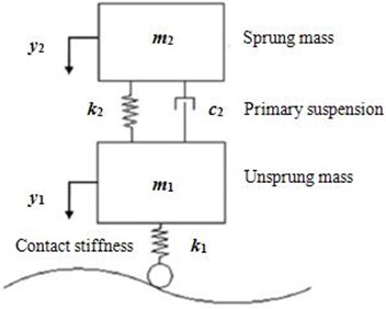
where is the amplitude and is the harmonic load frequency of the -th load. The static load is defined by and is equal to the load applied by a single train axle and , in order to simulate the permanent action of this static load. Dynamic loads are produced by wheel-rail contact irregularities and they have been obtained using an auxiliary quarter car model of the vehicle (see Fig. 2). This process is explained in [1].
Fig. 2Quarter car model used to obtain dynamic loads
Once the railway section is modeled and acting forces are defined, the following boundary conditions must be set:
where is the horizontal displacement of layer at depth , is the vertical displacement of layer at depth , is the horizontal stress of layer at depth and is the vertical stress of layer at depth . is the vertical displacement of the Timoshenko beam.
Furthermore Eq. (1) must be expressed in terms of Lamé and potentials in order to enable its solution. Thus displacements and stresses in horizontal and vertical directions are as follows:
Applying Fourier transform to Equations (1), (5), (6), (7), (8), (9), they are expressed in frequency and wave number domains and this leads to an algebraic system, which can be solved by mathematical tools. This process is detailed in [1].
The resulting accelerogram must be calibrated and validated with measured real data. The parameters which must be calibrated are * parameters of layers 1, 2 and 3, after a sensitivity analysis as is explained in [1]. The values of parameters once calibration and validation has been performed are listed in Table 1.
Table 1Analytical model parameters after calibration
Parameter | Layer 1 | Layer 2 | Layer 3 |
* | 450000 | 400000 | 525000 |
4. 3D FE model
The numerical model used for the study of wave generation and propagation caused by rail traffic is based on three-dimensional finite element method. Previously this methodology has been defined in [2]. In this case, as stated above, the section of track to be modeled is a conventional ballasted track with wooden sleepers located in the line of Santander-Liérganes operated by FEVE.
The software used to perform finite element model is ANSYS Product Launcher. The proposed dynamic problem solving is based on solving Eq. (10):
where is the global mass matrix, is the damping matrix, is the stiffness matrix, is the vector of displacements, is the vector of velocities and is the vector of accelerations.
Rayleigh damping theory is considered to generate the damping matrix as is shown in Eq. (11):
where and are the Rayleigh coefficients required to solve the dynamic analysis.
Considering the same hypothesis of the analogy to single-degree-of-freedom systems and the assumption that mass component is not influential in this type of phenomenon, damping matrix is calculated as:
being the modal damping ratio and the -natural modal frequency of the system.
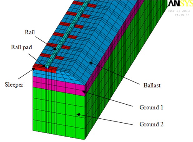
Railway structure modeling has been performed considering that action loads are vertical (axle load and dynamic loads caused by wheel-rail defects). Hence mechanical properties and geometry of the different elements are modified to match vertical inertia and rigidity of modeled materials with the real components of railway structure. A view of the 3D model is shown in Fig. 3.
Fig. 3Mesh and different elements of the simplified FE model
Dimension of the finite element model and the elements which compose it, wave propagation criterion have been established. Frequency range of 2-50 Hz has been set to study railway vibration phenomenon, since this range covers the large part of relevant frequencies in the whole body perception. Considering the prevalence of Rayleigh waves in ground surface vibration and the assumptions described in [2], the minimum length of the entire model is 47 m. As the model is applied to a conventional line, 60 is the minimum number of sleepers which respect this limiting length. Likewise the maximum length of elements must be up to 0.4 m. Note that symmetric conditions have been used to reduce computational time.
Once the model has been defined, a sensitivity analysis is necessary to fix the determinant parameters of the process. This analysis will provide the influential parameters which come into play in calibration and validation. Unknown parameters are the global Rayleigh coefficient and the elastic properties of ballast and top and bottom ground stratum.
As can be observed in the Figures 5, 6 and 7, Youngs modulus of ballast of top ground stratum and Rayleigh coefficient have a hard influence to the response acceleration of the model. These parameters have been calibrated and validated with real surface acceleration obtained from the measurement campaign. The calibration and validation procedure is detailed in [2]. Finally the resulting values of parameters after calibration and validation are listed in Table 2.
Fig. 4Acceleration response at surface for different ballast Young’s modulus values (E): a) E= 4.5·106 Pa, b) E= 8·106 Pa, c) E= 2·107 Pa, d) E= 7.5·107 Pa
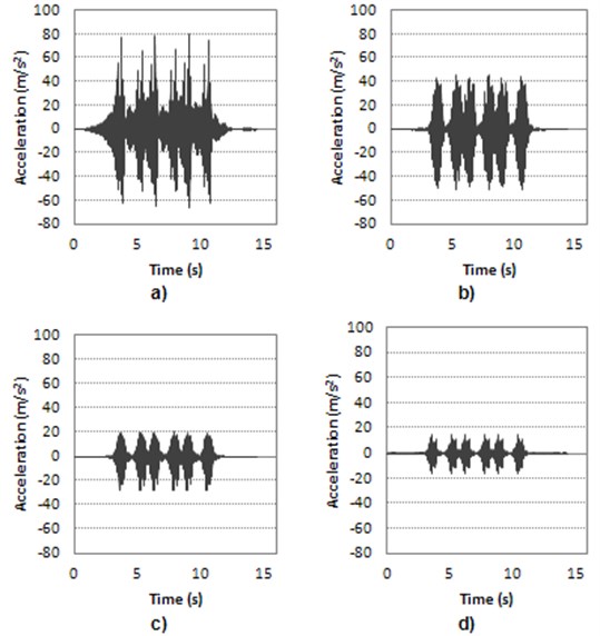
Fig. 5Acceleration response at surface for different top ground stratum Young’s modulus values (E): a) E= 5·106 Pa, b) E= 8.5·106 Pa, c) E= 1·107 Pa, d) E= 4.5·107 Pa
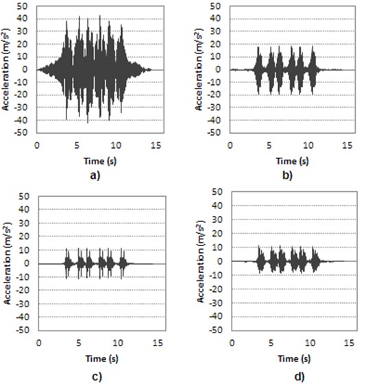
Fig. 6Acceleration response at surface for different β Rayleigh coefficient values: a) β= 0.0001, b) β= 0.0005, c) β= 0.001, d) β= 0.01
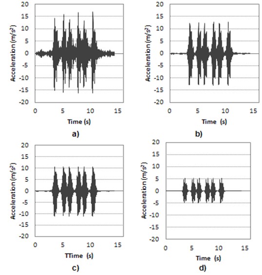
Table 2Calibrated values of influential parameters
Parameters | Calibrated values |
Rayleigh coefficient | 0.0005 |
Ballast Young modulus | 8·106 Pa |
Top ground stratum Young modulus | 8.5·106 Pa |
5. Comparison
Once analytical and numerical models have been developed, the following section addresses the comparison of both methodologies. First a theoretical comparison is carried out, analyzing the design hypothesis of each one, the differences between them and their limitations. After that the solutions obtained for the line of study by both models are compared. Moreover both models represent a useful tool to study vibration of different elements of the railway infrastructure in order to study how they are affected by traffic.
5.1. Theoretical comparison of the methodologies
Some theoretical considerations of both analytical and numerical models are presented.
First of all, considering the indispensable discretization of finite element models and neglecting other design simplifications, the most accurate solution is provided by analytical method, since it does not perform a discretional domain.
The application domain is one of the differentiation aspects between both methodologies. On one hand the analytical model is based on the establishment of the wave equation as a motion equation for each layer. This equation is applicable in two dimensions. Therefore the model domain is limited to the plane which contains track axis. Thus ground vibration can be only studied in longitudinal and depth directions. This way it is possible to study generation of vibrations. However, as it is a two-dimensional model, it is not capable to predict the phenomenon of wave propagation through the ground and how this affects to nearby structures. Therefore the analytical model is a powerful tool to study generation mechanism of ground vibrations caused by trains, but it cannot study wave propagation. Related to finite element model, it is a three-dimensional model and thus it is able to study generation as well as propagation of waves. It therefore shows an important advantage over the analytical model.
Regarding the input loads, analytical model applies a dynamic formulation. It introduces acting loads as a set of simple harmonic functions, including static load, with its special characteristics described previously. Numerical model requires load steps to represent the dynamic nature of acting loads. Load steps are applied in the nodes of the model that constitute the rail.
Related to frequency range of study, analytical model has no restrictions, meanwhile numerical model has a specific design for a frequency range of 2-50 Hz. In the event that a frequency out of range would be studied, a complete reformulation of the model would be required. The dimensions of the elements should be recalculated as well as the input loads, since load steps are dependent on the distance between the nodes. Train speed presents similar limitations for the range of frequencies in 3D FE model.
Table 3 presents a summary of the considerations stated above.
Table 3Summary of theoretical comparison of analytical and FEM models
Analytical model | 3D FE model | |
Solution | Exact solution | Approximate solution |
Degrees-of-freedom | Infinite degrees-of-freedom | Finite degrees-of-freedom |
Domain | Solution in the whole domain | Solution in the nodes |
Model | 2D model | 3D model |
Input loads | Dynamic formulation | Load steps |
Frequency range | Unlimited frequency range | Frequency range: 2-50 Hz |
Train speed | Unlimited train speed | Limited train speed |
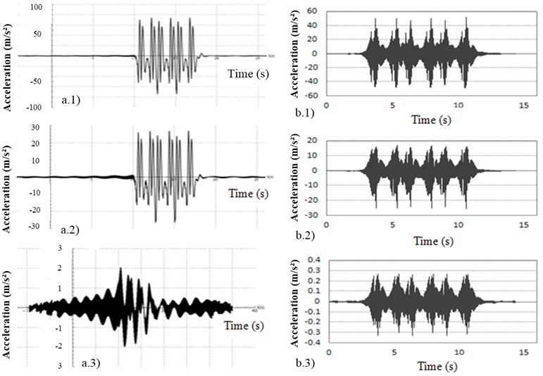
Fig. 7Acceleration response: a) analytical model: a.1) ballast, a.2) top ground stratum, a.3) bottom ground stratum; b) 3D-FE model: b.1) ballast, b.2) top ground stratum, b.3) bottom ground stratum
5.2. Comparison of results and simulations
There is an analogy between the viscoelastic parameters of the analytical model and damping coefficient of the numerical model. Both factors provide the damping characteristics model of the vibrations generated on the rail. Above all there is the correlation between and , which determines the vertical vibration response models. As these parameters are lower, the damping properties of the vibration wave also decrease, so that the vibration level increases, both on the surface and in depth. Also in this case the resulting ground motion is more diffuse. This is because the vibrations are attenuated with more difficulty and it takes longer to dissipate them.
Both analytical and numerical models have been calibrated and validated using surface acceleration data. Moreover some simulations of ground acceleration at different elements of railway infrastructure have been carried out. The results obtained by these simulations can be observed in Fig. 7.
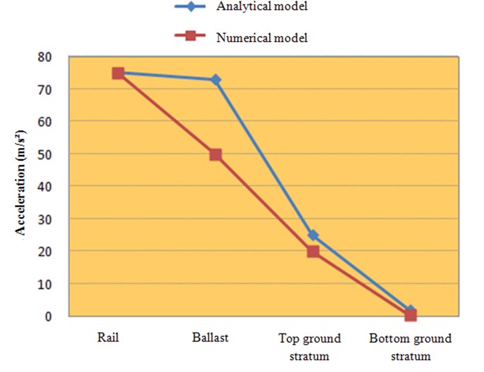
Focusing on peak simulated accelerations in each element, other conclusions can be obtained. In Fig. 8 it can be seen that peak accelerations obtained by numerical model are lower than the analytical ones. Furthermore analytical model cannot practically differ between rail and ballast acceleration, while numerical model is capable to do it.
Fig. 8Comparison of peak simulated accelerations of rail, ballast, top ground stratum and bottom ground stratum
6. Conclusions
The paper has properly developed both analytical and 3D-FE model to predict ground vibrations caused by railway traffic. Analytical model as well as numerical model are both able to evaluate vibration levels of the railway infrastructure.
Furthermore 3D-FE model can analyze the wave propagation phenomenon through ground surface. This is the most important advantage with respect to the analytical model.
Moreover both models represent a useful tool to study vibration of different elements of the railway infrastructure in order to study how they are affected by traffic.
References
-
Real J. I., Asensio T., Montalbán L., Zamorano C. Analysis of vibrations in a modeled ballasted track using measured rail defects. Journal of Vibroengineering, Vol. 14, Issue 2, 2012, p. 880-895.
-
Real J. I., Galisteo A., Real T., Zamorano C. Study of wave barriers design for the mitigation of railway ground vibrations. Journal of Vibroengineering, Vol. 14, Issue 1, 2012, p. 408-422.
-
Gutowski T. G., Dym C. L. Propagation of ground vibration: a review. Journal of Sound and Vibration, Vol. 49, Issue 2, 1967, p. 179-193.
-
Verhas H. P. Prediction of the propagation of train-induced ground vibration. Journal of Sound and Vibration, Vol. 66, Issue 3, 1979, p. 371-376.
-
Kurweil L. Ground-borne noise and vibration from underground rail systems. Journal of Sound and Vibration, Vol. 66, Issue 3, 1979, p. 363-370.
-
Krylov V. V., Dawson A. R., Heelis M. E., Collop A. C. Rail movement and ground waves caused by high-speed trains approaching track-soil critical velocities. Proceedings of the Institution of Mechanical Engineers, Vol. 214, Issue 2, 2000, p. 107-116.
-
Metrikine A. V., Vrouwenvelder A. C. W. M. Surface ground vibration due to a moving train in a tunnel: two-dimensional model. Journal of Sound and Vibration, Vol. 234, Issue 1, 2000, p. 43-66.
-
Koziol P., Mares C., Esat I. Wavelet approach to vibratory analysis of surface due to a load moving in the layer. International Journal of Solids and Structures, Vol. 45, Issue 7-8, 2008, p. 2140-2159.
-
Zou J.H., Feng W. X., Jiang H. B. Dynamic response of an embedded railway track subjected to a moving load. Journal of Vibroengineering, Vol. 13, Issue 3, 2011, p. 544-551.
-
Cirianni F., Leonardi G., Scopelliti F. Study of the barriers for the mitigation of railway vibrations. The Sixteenth International Congress on Sound and Vibration, Kraków, 5-9 July 2009.
-
Salvador P., Real J., Zamorano C., Villanueva A. A procedure for the evaluation of vibrations induced by passing of a train and its application to real railway traffic. Mathematical and Computer Modelling, Vol. 53, Issue 1-2, 2010, p. 42-54.
-
Real J. I., Maartínez P., Montalbán L., Villanueva A. Modelling vibrations caused by tram movement on slab track line. Mathematical and Computer Modelling, Vol. 54, Issue 1-2, 2011, p. 280-291.
-
Andersen L., Jones C. J. C. Three-Dimensional Elastodynamic Analysis Using Multiple Boundary Element Domains. ISVR Technical Memorandum, University of Southampton, 2001.
About this article

