Reliability assessment based on an adaptive response surface method considering correlation among random variables

2.1. Diverging example

To analyze this type of problem, a face slab of a Concrete Face Rock-fill Dam (CFRD) has been selected (see Fig. 1). Such a section of the continuous slab is considered as a cantilever beam for the analysis, being the support the lower part. With the setting of a combination of fixed and seismic load equivalent to 0.154 g, the maximum moment external loads at the critical location of the cantilever beam were calculated with Strand-7, a commercial finite element program.

The continuous face slab of the target CFRD dam is supported by uniformly compacted foundation. Hence the settlement of structure will be ignorable. The material model is mainly composed of 24 MPa compressive strength concrete and reinforcements of 300 MPa ultimate strength, which limits surface crack in terms of over 0.4 % reinforcing volume ratio. The material, structural and geometric information for the selected elements are like the following Fig. 1. As can be seen, the maximum moment was 8.51 kN-m.

Fig. 1a) FE Model, b) resultant factored external moment of the example structure

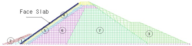
a) Mesh for FE Model

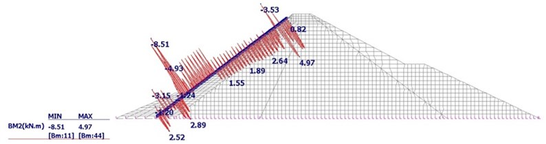
b)$M_{max}=$51 kN-m

Next, three axial points were chosen to construct the response function with a gap of ± (standard deviation) between center points (the average of random variables), and axial points. The performance of the target beam was then calculated using the LSFs for estimating the probability of flexural failure, when the value of the function is less than or equal to zero.

A maximum crack width is now calculated in order to predict the probability for this width to exceed the design criteria. To do so, a response surface based on a quadratic RSM has been utilized, and compared with the results of both MCS and FOSM. Under an external service moment of 7.30∙10⁶ kN-mm at the critical location of the cantilever beam, the serviceability LSF for the crack width was evaluated as:

where:

$t_c=\frac{diameter\mathrm{}of\mathrm{}reinforcement}{2}=10.50\text{mm},$

$d_{c,\text{min}}=the\mathrm{}minimum\mathrm{}cover\mathrm{}depth=20\text{mm},$

$\beta =(H-k\cdot D)/(D-k\cdot D)=1.068,$

$H=theheightofthebeam,$

$k=-np+\sqrt{{\left(np\right)}^2+2np}=0.229,$

$p=0.003775,$

$n=ratio\mathrm{}of\mathrm{}elasticity\mathrm{}of\mathrm{}steel\mathrm{}and\mathrm{}concrete=E_s/E_c=200000/\left(4700\sqrt{f_{ck}}\right)=9,$

$f_{ck}=the\mathrm{}28th\mathrm{}day\mathrm{}compressive\mathrm{}concrete\mathrm{}strength,$

$D=depth\mathrm{}of\mathrm{}the\mathrm{}beam=400\text{mm},$

$f_s=thesteelstress=M_e/A_s\left(D-\frac{x}{3}\right)=14.518\text{MPa},$

$x=k\cdot D=86.930\text{mm},$

$A_s=the\mathrm{}confining\mathrm{}area\mathrm{}for\mathrm{}reinforcements=\frac{2\cdot dy\cdot B}{Number\mathrm{}of\mathrm{}reinforcements}=\mathrm{}8000\text{m}{\text{m}}^{\text{2}},$

$dy=d_{c,\text{min}}=20\text{mm}.$

Table 1 shows the random variables used in each case (where $M_e$ is the unfactored external moment), as well as their mean values and coefficients of variation (C.O.V.) assuming a normal distribution.

The performance of the target beam has been calculated using the LSFs presented in Eqs. (4) and (5), composed by a quadratic RSM as follows:

and the LSF for MCS or FOSM is:

where $g(\cdot )$ is again the LSF and ai represents the coefficients of the response function. Making use of the values calculated above, and assuming a 0.1 coefficient of variation for the $w_{allow}$, the statistical values of the selected random variables are estimated in Table 5. The load term in the LSF is evaluated by RSM+FOSM, FOSM, and MCS, equivalent to the expected maximum crack width calculated as $X_6$ in the same Table, following the Korean Concrete Institute recommendations.

The coefficients of the response surface constructed by a least square method, while varying the area of reinforcements in Table 2, are as follows:

The response surface functions (expressions in parenthesis in Eq. (6) are used as the demand terms in the LSFs. After constructing the LSFs of such Eq. (6), the reliability indices can be calculated by FOSM. In contrast, reliability indices for Eq. (6) were evaluated by MCS and FOSM. Three kinds of reinforcement areas are considered for varying demand terms in the LSFs. The compared results of RSM (+FOSM) against MCS and FOSM, show increased differences than those in the previous example (only 6 %), being now 53.4 % the maximum difference, when the reinforcement area is 351.9 mm² (see Table 3).

Again, this value compared with the results obtained earlier, related to the differences among the simulation methods, reveals bigger discrepancies between RSM (+FOSM) and FOSM (or MCS), mainly as a result of the increased nonlinearity in the LSF – Eq. (2) and Eq. (5).

In Table 3, the three different methods are used and compared for the evaluation of the same LSFs. This example shows the diverging issues already mentioned, which lead directly to the proposition of an improved RSM.

In Table 3, the negative reliability indices indicate that there are severe discrepancies between ultimate limit state and serviceability limit state. Note that the safety margin for the serviceability limit state is relatively low, due to the risk of the two events. Having analyzed these examples with traditional approaches, now one that overcomes the limitations of the previous two will be presented.

2.2. Bayesian belief network model (BBN)

The correlation among random variables for infra structures has been studied in a various way. The most well-known general modeling technique is event tree analysis (ETA) or fault tree analysis (FTA), which are convenient for qualitative analysis but hard to model for various sources. Markov process modeling overcame the weakness of ETA and FTA although it is not appropriate for modeling complex system.

The correlation modeling has been specifically dealt by bayesian update modeling technique. Since 1985, BBN could model a highly correlated causal system in an inductive way, which cannot determine the distribution of effects from results to cause direction. Therefore, the inverse way of BBN is proposed in this research in order to identify the role of random variables to consequential result considering correlation among random variables of each member.

BBN are a graphical structure known as a directed acyclic graph (DAG). A DAG is a set of nodes and arcs, or directed edges, between nodes, such that there is no directed cycle.

BBN is typically built by first finding an appropriate structure either by interviewing an expert, or by selecting a good model from training data, and then using a training sample to estimate the parameters (Darwiche, 2000). The resulting belief net is then used to answer queries based on joint probability.

Compared with event tree analysis (ETA) or fault tree analysis(FTA), BBN could evaluate and detect a partial failure in a probabilistic quantification, which is not allowed in ETA or FTA. It additionally overcome the exponentially increased complexity in stochastic modeling of Markov Model by employing zipping techniques. This feature is shown by showing superiority to Markov Chain Monte Carlo Simulation as well, i.e., Metropolis method or Gibbs Sampling in terms of simplification by zipping.

The steps of uncertainty analysis in a BBN model are as follows:

1) defines a set of random variables;

2) defines a joint distribution for these random variables;

3) defines other variables which are functions of the random variables;

4) Monte Carlo samples the entire joint distributions (probabilistic and functional variables);

5) communicates the probabilistic prediction results,

where, the random variables are assigned marginal distributions, followed by a specification of a DAG to capture conditional relations. Probabilistic influence between parent and child is represented as conditional rank correlation. A joint probability density for the probabilistic nodes is built using the joint normal copula to realize the dependence relations. This density can be updated analytically, or sampled and analyzed with Monte Carlo Simulations.

3.1. Improvement techniques

In spite of the two issues discussed before, the merits of the basic RSM are remarkable, and perhaps that is the reason why it has been widely applied for carrying out reliability analysis. The approximation of structural responses, however, would show relatively large errors depending on the nonlinearity form of the LSFs. Irfan et al. (2005) proposed a weighted regression method in which the response surface function was formulated by assigning higher weights to the variable that was closer to the limit state. To do so, they adopted an $n\times n$ diagonal matrix of weights and the best design, amongst the responses from the performance function corresponding to the design matrix, was selected. Consequently, the distance among input random variables is optimally determined. This occurs when the LSFs approaches to zero. Thus, the best response can be given as:

where ${\overrightarrow{f}}_{best}$ is the determined best value amongst the axis points, and $g{\left(x\right)}_i$ is the fitted response on the response surface, composed by center and axis points at the iteration step.

The component of the weighted matrix in each iterative calculation can be expressed in the following manner:

where $w_i$ is the component of the weighted matrix, and needs to be multiplied by the center or axis points, for composing an improved response surface for the next iterative step. Consequently, the longer arm length between axis points is reduced, providing closer design points than the old axis points.

To improve the convergence and accuracy when dealing with nonlinear LSFs, a first approximation could be to integrate the weighted matrix with the adaptive iteration developed by Rackwitz-Fiessler, leading to the establishment of the adaptive weighted response surface (AWRS) function. However, having combined the improved techniques (both linear and nonlinear response surface functions using basic, adaptive, and adaptive weighted method) the authors concluded that the linear adaptive weighted response surface method (LAW-RSM), was the best alternative. The following examples are aimed at demonstrating this statement.

3.2. Validation of the LAW-RSM

The random variables in the example of the simply supported beam selected for analysis are: distributed load (W), span length (L), modulus of elasticity (E), and the moment of inertia (see Fig. 2).

Fig. 2Scheme of the beam considered in Example 1

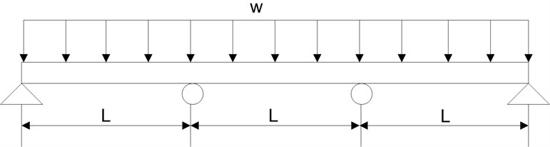
The limit state being considered is deflection, and the allowable deflection is specified to be $L/360$. The maximum deflection is $0.0069W{L}^4/EI$, and it occurs at $0.446L$ from either end of the beam.

The limit state function is:

The mean and coefficient of variation for each of the variables under study are presented in Table 4.

In the example considered, the linear RSM was accurate with the weighted regression method. As can be seen in Table 5, while the application of the quadratic LAW-RSM resulted in a difference of 42.23 %, compared with the results of the classical MCS, the LAW-RSM showed less than 3 % of difference with such a simulation approach. However, the convergence and accuracy will be changed depending on the linearity order of limit state function.

3.3. Correlation model for random variables in BBN

BBN were a convenient alternative to develop the model. They are graphs, whose nodes are connected by arcs. While nodes represent variables, arcs represent the strength of the relationship between them (Hanea, 2008). The employed bayesian belief net is answer queries for the following probability density function based on conditional probability:

Following Markov condition for BBN (chain rule) the above joint probability is then calculated as:

where, $P_{xy}$ is a coefficient of correlation between random variables, $x_i$ and $u_i$denotes each random variable, $n$ represents the total number of random variables, $S_x,S_y$ are standard deviation of variables, and $\stackrel{-}{x},\stackrel{-}{y}$ are mean value of random variables.

Four variables were considered as important for the model, they are: (i) moment of inertia, (ii) elasticity, (iii) distributed load intensity and (iv) length of a span (see Table 4). The analytical conditioning in BBNs on four probabilistic nodes can be conditionalized, whereby the conditional distribution is computed in a few minutes. This is possible with the joint normal copula. Random variables are treated as transformations of joint normal variables.

If $Z=(Z_i,...,Z_n)$ denotes a joint normal distribution of normal variables $Z_i$ with mean zero and unit variance, then random variables $X_i,...,X_n$ are written as

where $F_i$ is the cumulative distribution function of random variable $X_i$, and $F_n$ is the cumulative distribution function of the standard normal variable. If $F_i$ is continuous invertible, this transformation is rank preserving, the rank correlations of $X_i$, $X_j$ will be the same as that of $Z_i$, $Z_j$.

The rank correlation of normal variables is computed from the product moment correlation with the Pearson transformation. For details see (Hanea et al., 2006)

Conditioning on the value $X_i=x$ entails conditioning $Z$ on $Z_i={\Phi }^{-1}\left(F_i\right(x\left)\right)$. Letting $Z(X_i=x)$ denote this conditional distribution, the conditional distribution of $X_i,...,X_n$, when $X_i,...,X_n$ are joined by the joint normal copula, is given by:

The results of conditioning among random variables could be presented in graphical format in various ways. As showin in Fig. 3, if used with the results of Monte Carlo simulation, it may be hard to understand due to the complex correlation.

Fig. 3Correlation among random variables shown in Cobwebs

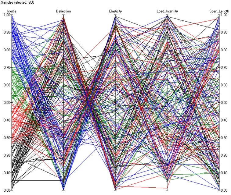
Fig. 4a) BBN model among random variables, b) probability density function of each varibale

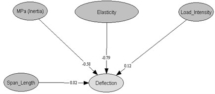
a)

b)

Therefore we have selected quantified regression analysis between two variables. One of the most important variables in structural analysis would be deflection. The correlation between deflection and other variables are investigated presented in Fig. 4 and Fig. 5. By the results, it turns out that due to the contribution of span length to the load intensity the correlation between deflection and span length show the largest sensitivity while modulus of elasticity show the lowest correlation, shown in Figure 5. This is quite different with simply supported beam case, where deflection is directly proportional to Moment load while it is reversely proportional to elasticity of modulus times inertia of secondary moment of the sections.

Consequently, while the proposed improved RSM method could present faster converged and improved evaluation of reliability of structures, Bayesian belief net model additionally provide contribution of each random variables in terms of correlation among components.

Fig. 5Correlation and conditional expectation of deflection on other random variables

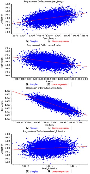
a) Correlation of defl ection on random variables

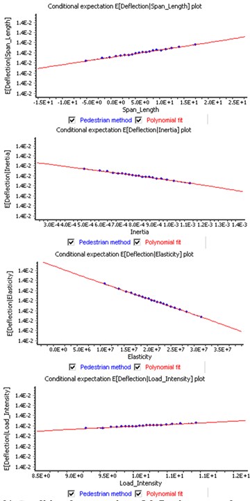
b) Conditional expectation of deflection on random variables