Investigation of fling-step effect on the selected structures subjected to the simulated Fandoqa near source strong motion

1. Introduction

Near source ground motion poses two significant earthquake charactristics;"forward directivity" and "permanent displacement". The former is as the cause of arriving the greater part of energy from the rupture to a single coherent long-period pulse at the site and the latter is resulting from unidirectional tectonic movement. Such motions may generate high seismic demands (Kalkan and Kunnath [1]). The destructive effects of near-source earthquakes have been distinguished during a number of worldwide earthquakes, e.g., Landers (USA, 1992), Northridge (USA, 1994), Kobe (Japan, 1995), Fandoqa (Iran, 1998), Kocaeli (Turkey, 1999), and Chi-Chi (Taiwan, 1999). Despite numerous studies done on the field of forward directivity effects on seismic demands, a limited number of research works is found in the context of the fling step contribution to seismic demands of structures. The reason might be due to the scarcity of as-recorded ground motions being associated with the fling step contribution in particular at both sides of the causative fault. For this reason, we simulated seismograms, including fling step effects, at both sides of the causative fault aimed at better understanding the circumstance under which the static permanent displacement affects the seismic demands.

The renewed Fandoqa (1998) earthquake of Iran is chosen as a case study. The optimal seismological parameters of the causative fault are estimated through developing an inversion solution technique by means of an evolutionary approach with the specific objectives. Noteworthy, since fling step is often associated with long period pulse, the structures under study should also have sufficiently long fundamental period so that the problem would be better understandable. The results of this research work are expected to give a general insight into the problem for extrapolating the trouble to the north parts of Tehran city where are likely to be threatened by near source strong motion including fling step effects.

2. Ground motion simulation methods

Reproducing near source ground motion, within the last decade, accounting for the forward directivity effects have been well published (e.g., [2-4]). However, still too much work is needed in the field of such waveforms in particular those being influenced by forward directivity and fling step. Generally speaking, synthetic seismograms may be categorized as: a) Omega-squared-based ground motions such as point source [5, 6] and finite fault methods [7, 8], b) Green’s function-based methods, either in the form of empirical [9-12] or theoretical [13-16], and finally c) hybrid methods [17, 18]. In this study the theoretical Green’s function-based form proposed by Hisada and Bielak [15] is employed to reproduce the main event at Sirch station of Fandoqa (1998) scenario, the most famous near source earthquake around the region under study at which the as-recorded data is influenced by forward directivity and fling step.

3. Reproducing the causative event Fandoqa scenario (1998) at Sirch station

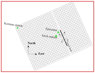
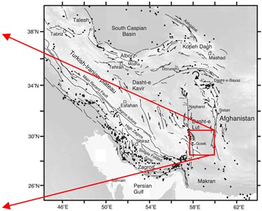
At March 14 (1998), a strong strike-slip earthquake of Mw 6.6 occurred in Kerman state located at the South-Eastern part of Iran. Approximately five people were killed in Golbaf, 50 were injured, 10000 become homeless and 2000 houses were destroyed [19]. This earthquake ruptured about 20 km of the Gowk fault system. Fig. 4 shows the active faults of Iran along with that of the Gowk fault system. The location of the selected stations near the Gowk fault named St-1, St-2, St-3, and St-4 are also shown.

The theoretical-based Green’s function method (TGF) proposed by Hisada and Bielak [15] is employed for reproducing the as-recorded ground motion at Sirch station with focusing on the long period pulses associated with the seismogram ($f\le$1.5 Hz). This record has already been reported to be associated with forward directivity and fling step effects [20]. As a consequence, we only need to extract the fling step from the original seismograms so as to better understand the fling step contribution to seismic demands. For this purpose, Iwan’s method [21] is adopted, as the first step, to correct the raw data and the Abrahamson’s approach is used for determining the pulse duration corresponding to the fling step as the second step. This method of removing fling step effects from the seismograms ensures that the forward directivity effects associated with the waveforms remains saved.

Numerous types of evolutionary-based techniques are available in the literature for solving such problem (e.g., [22-24]). Among the existing approaches, the sigma method [25] due to its ability in finding solutions with very good diversity and high convergence potentiality is employed. To this end, a Multi-Objective Particle Swarm Optimization algorithm (MO-PSO) including an inversion solution technique is developed. The MO-PSO evolutionary-based algorithm used includes the three objective functions: response spectra corresponding to the three components of seismogram (horizontal east-west, north-south components, and vertical component), and multi-taper spectra [26, 27] (was intended to match the frequency content). A MTLAB code is written by which the defined error functions reflecting differences between the response spectra corresponding to the simulated and the as-recorded data are minimized. The site soil conditions reported by BHRC [28] are incorporated into the developed model. Eqs. (1), (2) and (3) show the definition of the objective functions used in this study:

where $SP$, $MT$, $ob$ and $sim$ represents response spectrum, multi-taper spectrum, observed and simulated respectively. $n_{sp}$, $n_{MT}$ denote number of points of response spectrum and multi-taper spectrum. K denotes on North, East and Vertical components. The objective functions, treating independently, are iteratively calculated through producing waveforms followed by calculating their residual errors. This procedure were continued untill the predefined convergence criteria is achieved. The upper-lower parameter values of the unknown model parameters are required to be already defined in the algorithm. This type of inputting data enables the evolutionary-based approach to be processed within the pre-defined range of seismological model parameters at the expense of time cost. The best such limitation of the input parameters are those already suggested by the other investigators for this causative fault. In the context of the model parameter type, the triangular slip function model with four time-windows is adopted and incorporated into the model. With this information in hand, the program was run and the optimal seismological model parameters such as: the length, the width, strike, dip, rake, slip, rupture velocity, hypocenter location were obtained. The calculation processing were paused as a series of the results termed "non-dominated Pareto front" associated with different error levels were obtained. In this stage, all of the obtained model parameter sets are interpreted as the feasible solution for the problem. However, a limited numbers are selected as the most appropriate model parameters. Table 1 lists the obtained optimal values of model parameters along with those previously suggested for Fandoqa scenario by the other investigators. As seen, the obtained parameters are in consistent with those of the others confirming somehow the acceptability of our model parameters. A comparison between the obtained synthetic and those of the real seismogram (as-recorded) in terms of acceleration and response spectra are shown in Figs. 1-3.

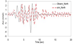
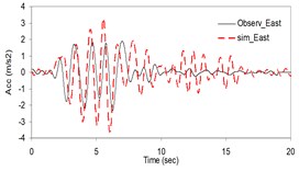
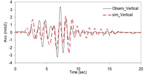
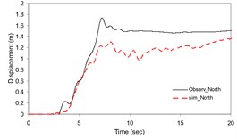
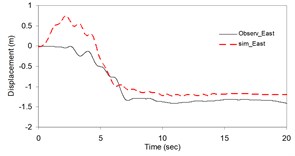
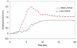
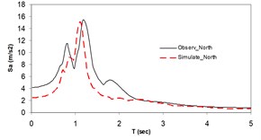
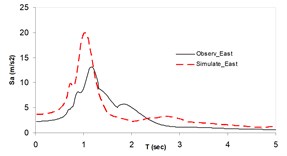
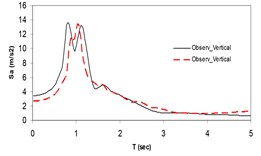
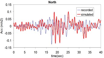
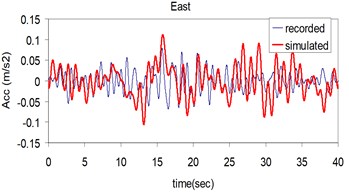
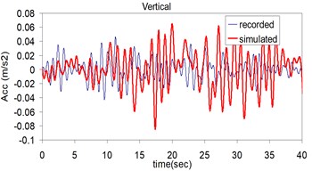
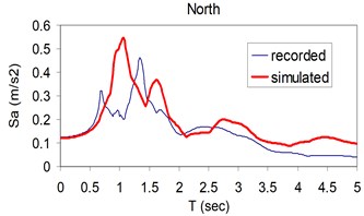
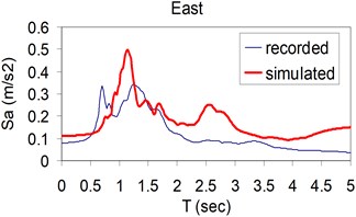
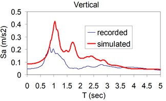
As the validation step, the model was calibrated by incorporating the obtained optimal parameters into the model and extrapolating the simulation process to the other station (Kerman station) where the causative event has been recorded (see Fig. 4). Consequently we arrived at providing the synthetic waveforms at the two stations, Sirch which has been influenced by the forward directivity and fling step effects while Kerman has not been affected by fling step. Fig. 1 demonstrates the simulated and recorded three component acceleration time-histories (North, East, and Vertical) at Sirch station. The comparison of the three components of the simulated and the as-recorded displacement time-histories are shown in Fig. 2. Fig. 3 displays the comparison of the three components acceleration response spectra corresponding to the simulated and recorded seismograms at Sirch station. Fig. 5 displays the simulated and the recorded ground motion time-histories at Kerman station. The response spectra corresponding to those at Fig. 5 are shown in Fig. 6. As seen, acceptable comparison of the simulated and recorded model parameters as well as the seismograms ensure the reliability of the model in synthesizing this event at sites around these two stations.

Fig. 1Plots of the simulated and recorded three component acceleration time-histories (North, East, and Vertical) at Sirch station

a)

b)

c)

Fig. 2Plots of the simulated and recorded three component (North, East, and Vertical) displacements at Sirch station

a)

b)

c)

Fig. 3Plots of the simulated and recorded three component (North, East, and Vertical) waveform's response spectra at Sirch station

a)

b)

c)

Fig. 4a) Location of the selected stations namely St-1, St-2, St-3, and St-4 near the Gowk fault alignment and b) the active faults of Iran

a)

b)

Fig. 5Plots of the recorded (thin) and simulated (thick) three component acceleration time history (North, East and Vertical) at Kerman station

a)

b)

c)

Fig. 6Plots of comparison of the response spectra corresponding to the simulated (thick) and recorded (thin) three components (North, East and Vertical) at Kerman station

a)

b)

c)

Fig. 73D alignment of Gowk fault [29]

4. Studied structural models

The contributions of fling-step to seismic demands are studied using the two selected structures, a steel structure and a reinforced concrete frame. As mentioned earlier, the reason of selecting these two buildings are that the fundamental period of the structure being evaluated against fling step should be sufficiently long because fling-step is often associated with a long-period pulse. The first structure is a 30-story dual system (MRF and X-brace) steel building designed based on the ASCE-07-10 [30] and AISC-ASD 89 code. The plan and elevation of the studied building are shown in Fig. 8. The columns and braces sections are box form while those of the beams are IPE profile. The height of structure and bay length along X and Y directions are 3, 4 and 5 m respectively. The three dimensional form of the 3D structure subjected to the obtained synthetic waveforms was carried out using SeismoStruct ver. 6 software [31]. The maximum inter-story drifts were calculated performing a series of nonlinear dynamic analysis. The natural periods of the structure are listed in Table 2. The second structure is a 20-story special RC frame previously designed based on the ASCE7-02 and ACI318-02 code (Haselton and Deierlein, [32] building ID 1020). Details of the 2D frame are found at [32]. This structure is modeled and dynamically analyzed using the well known Opensees software [33].

Fig. 83D elevation, plan and section of the studied 30-story dual system steel structure

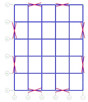
a) Plan

b) Elevation

Fig. 92D 20-story special R/C frame ID 1020, Haselton and Deierlein model [32]

It is worth mentioning that, the contribution of fling step to seismic demands needs a series of waveforms with and without fling step effects. Therefore, we need to compute the fling pulse durations corresponding to the N-S and the E-W components of seismograms at the selected four stations. For this purpose, a brief explanation on the computing the simple fling-pulse type model and removing the obtained fling step time-histories from the original waveforms are presented in the next section.

4.1. Removing the fling step pulses from the original waveform

There are limited numbers of trusty methods considering the extraction of forward directivity pulse period coupled with fling-step time-history in the literature (e.g., [34, 35]). The method introduced by Abrahamson [34] was adopted in this study due to its simplicity and capability of monitoring the required parameters for simple-pulse-type modeling of the fling step. Two key parameters are computed for both components of each ground motion pair: a) step duration ($T_{pf}$) and b) the time from which the fling step pulse is initiated. In this method, a straight line connecting the flat sections of the both sides in the displacement time-history is drawn. The intersection of the straight line and the two flat sections gives the value of $0.8T_{pf}$ associated with the permanent static displacement. Fig. 10 typically shows the extracted fling step permanent static displacement $D$ and associated pulse period $T_{pf}$.

Fig. 10Graphical illustration of Abrahamson’s model for determining fling step permanent displacement D and pulse period Tpf [34]

The computed $D$, $T_{pf}$ and pulse arrival time, $t_i$, are incorporated into the simple pulse-type fling step proposed by Kalkan and Kunnath [1] thus obtaining the fling step in time-history form. In the next step, the fling step effects included in the synthetic seismograms are extracted by subtracting the fling step simple pulse-type model from the synthetic waveforms. The mathematical form of the fling step pulse acceleration model used is expressed as:

4

$a\left(t\right)=\frac{2\pi D}{T_{pf}^2}\sin \left(\frac{2\pi }{T_{pf}}\left(t-t_i\right)\right),t_i\le t\le T_{pf},$

where $T_{pf}$, $t_i$ and $D$ are: fling step pulse period, pulse arrival time, and permanent displacement respectively. The fling-step pulse period of waveforms at stations 1, 2, 3 and 4 are listed in Table 4.

Table 4Fling-step pulse period of the synthesized waveforms

Station No.	St-1	St-2	St-3	St-4
$T_{pf}$ (sec)	1.3	3.9	4.5	3.5

5. Time-history analysis of the buildings subjected to the synthesized waveforms and results

The synthesized strong motions were generated at four stations, with two stations at each side close to the causative fault. These synthetic ground motions were in the forms of with and without fling step effects. Therefore eight series of the synthetic ground motions were used in the dynamic analyzing process. The two NS and EW horizontal components of the synthetic ground motions at the four stations were simultaneously applied to the 3D dual system steel structure whereas the single NS and EW components were independently applied to the 2D R/C special moment frame. The SeismoStruct [31] and Opensees software [33] are used for dynamic analysis of the 3D and 2D structures respectively. The maximum inter-story drifts corresponding to the both principal directions ($X$ and $Y$) in the 3D structure and that of the 2D frame are calculated performing a series of dynamic nonlinear analysis. The results at each station are discussed in the subsequent sections.

5.1. Results at station No. 1

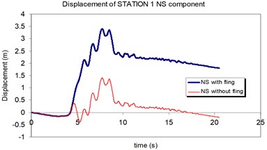
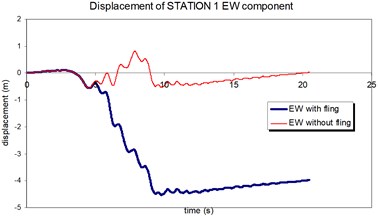
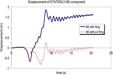
The displacement time-histories corresponding to the horizontal NS and EW components at station No. 1, with and without fling step contribution are shown in Fig. 11. Fig. 12 displays the acceleration response spectra corresponding to these two components with and without fling step contribution at this station. The seismic demands of the 30 story structure subjected to the two horizontal components of the synthetic waveforms (NS and EW) at station No.1 are demonstrated in Fig. 13. The EW and NS components of the synthetic ground motions at station No. 1 were independently applied to the 2D frame which already has been used by Haselton and Deierlein [32]. Fig. 14 displays the MISDRs (Maximum Inter-stories Drift Ratios) over the height of this structure. As seen, the contributions of fling step to seismic demands are different in the two directions $X$ and $Y$ and also different throughout the height of the structures. The differences are from smaller to larger seismic demands confirming that, fling step contribution to seismic demands cannot be predicted.

Fig. 11Comparison of the displacement time-histories with and without fling step contribution at station No. 1, a) NS component, b) EW component

a)

b)

Fig. 12Comparison of the response spectra with and without fling step contribution at station No. 1, a) NS component, b) EW component

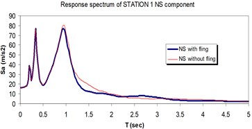
a)

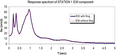
b)

Fig. 13Comparison of the seismic demands at the 3D-30 story structure with and without fling step contribution at station No. 1, a) max inter-story drift in Y direction, b) max inter-story drift in X direction

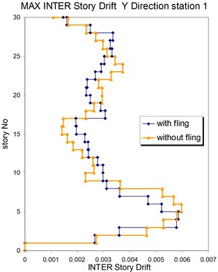
a)

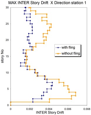
b)

Fig. 14Comparison of the seismic demands at the 2D-20 story frame with and without fling step contribution at station No. 1, a) maximum inter-story drift at NS component, b) maximum inter-story drift at EW component

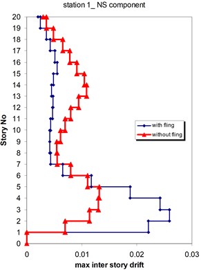
a)

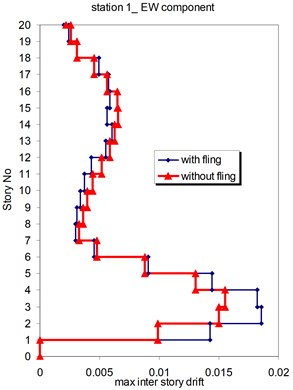
b)

5.2. Results at station No. 2

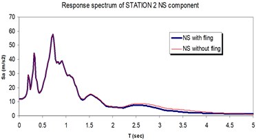
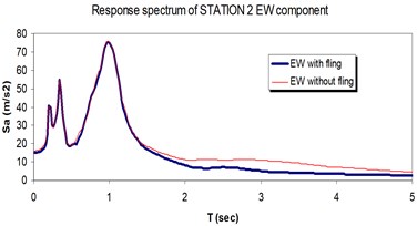
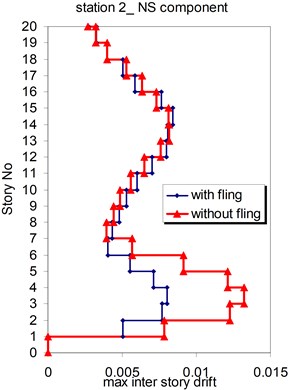
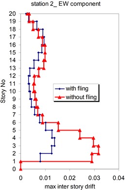
The above mentioned calculations and plotting were repeated at station No. 2 and the MISDRs over the two structures were obtained. As seen, the contribution of fling step in seismic demands can't be previously predicted because is different in different direction and stories.

Fig. 15Comparison of the displacement time-histories with and without fling step contribution at station No. 2, a) NS component, b) EW component

a)

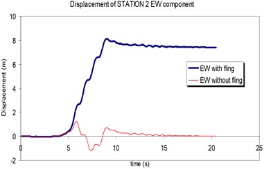
b)

Fig. 16Comparison of the response spectra with and without fling step contribution at station No. 2, a) NS component, b) EW component

a)

b)

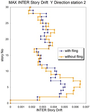
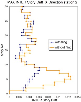
Fig. 17Comparison of the seismic demands with and without fling step station No. 2, a) max inter story drift of the 30-story structure for Y direction, b) max inter story drift of the 30-story structure for X direction

a)

b)

Fig. 18Comparison of the seismic demands with and without fling step station No. 2, a) max inter story drift of the 20-story Haselton model for NS component, b) max inter story drift of the 20-story Haselton model for EW component

a)

b)

5.3. Result for station No. 3

The calculation process at the stations 3 and 4 were continued by applying the synthetic seismograms upon the two selected structures and calculating the MISDRs.

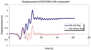
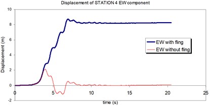
Fig. 19Comparison of the displacement time-histories with and without fling step contribution at station No. 3, a) NS component, b) EW component

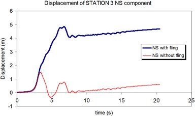
a)

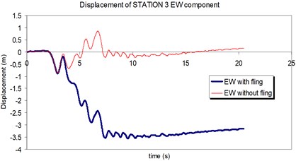
b)

Fig. 20Comparison of the response spectra with and without fling step contribution at station No. 3, a) NS component, b) EW component

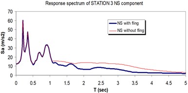
a)

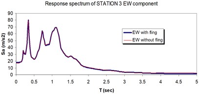
b)

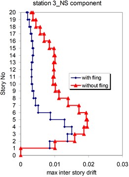
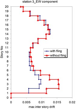
Fig. 21Comparison of the seismic demands with and without fling step station No. 3, a) max inter story drift of the 30-story structure for Y direction, b) max inter story drift of the 30-story structure for X direction

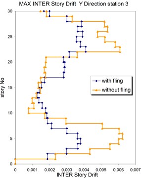
a)

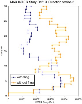
b)

Fig. 22Comparison of the seismic demands with and without fling step station No. 3, a) max inter story drift of the 20-story Haselton model for NS component, b) max inter story drift of the 20-story Haselton model for EW component

a)

b)

5.4. Result for station No. 4

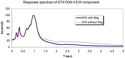
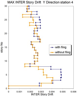
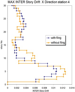
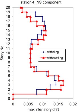
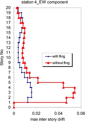
As seen in Figs. 21, 22 and 25, 26 at stations 3 and 4, the obtained results confirm that, there isn't evidence by which one can answer the question that, weather the fling step increase or decrease its contribution to seismic demands? In other words, the contribution of the fling step associated with the strong motion at near source sites to seismic demands as least at the above mentions circumstances is not predictable. This conclusion is in contrast to that of Kalkan and Kunnath [1] which claimed that, fling step highly increases the seismic demands of structures.

Fig. 23Comparison of the displacement time-histories with and without fling step contribution at station No. 4, a) NS component, b) EW component

a)

b)

Fig. 24Comparison of the response spectra with and without fling step contribution at station No. 4, a) NS component, b) EW component

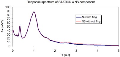
a)

b)

Fig. 25Comparison of the seismic demands with and without fling step station No. 4, a) max inter story drift of the 30-story structure for Y direction, b) max inter story drift of the 30-story structure for X direction

a)

b)

Fig. 26Comparison of the seismic demands with and without fling step station No. 4, a) max inter story drift of the 20-story Haselton model for NS component, b) max inter story drift of the 20-story Haselton model for EW component

a)

b)

6. Conclusion

The contributions of fling step to seismic demands of the selected two structures subjected to the synthesized near source strong motion including fling step effects are investigated. Due to the scarcity of the seismogram close to causative fault including permanent static displacement effects, in particular with the stations at the two sides of the causative fault, we used synthetic seismograms. Before entering into the problem, the three components of strong motions recorded at Sirch station (Fandoqa scenario, 1998) in Kerman province located at the south-east part of Iran were simulated The theoretical-based Green’s function method (TGF) proposed by Hisada and Bielak [15] were employed for generating synthetic strong motions. A Multi-Objective Particle Swarm Optimization algorithm (MO-PSO) was developed through which the differences between the as recorded and synthetic seismograms were minimized. Three objective functions representing the differences between the synthetic and real data were defined. This evolutionary processing came up with the optimal model parameter values such as: the length, the width, strike, dip, rake, slip, rupture velocity, hypocenter location. For the purpose of computing the permanent static displacement associated with the synthetic waveforms, the synthetic seismograms are corrected using Iwan’s method [21]. After ensuring the calibration of the simulation model, the obtained optimal parameters were incorporated into the model and the calibrated model was used for extrapolating the synthetic waveforms at the other four stations. Two structures, a 30-story dual system (MRF and X-brace) steel building and a 20-story special RC frame previously designed based on the ASCE7-02 and ACI318-02 code [32] were used. The SeismoStruct [31] and Opensees software [33] were used for modeling and dynamically analyze the selected structures. The Maximum Inter-stories Drift Ratios (MISDRs) over the height of the structures, as the results of applying the two types of synthetic seismograms, with and without fling step effects, upon the structure, were calculated. It was concluded that, in general, the fling step contribution to seismic demands is not a predictable problem in contrast to that of Kalkan and Kunnath [1] which expressed that, fling step increases the seismic demands. However, still much work is needed to better monitor the contribution of fling step to seismic demands under another circumstances e.g., irregular structures.