Abstract
A troublesome problem in application of local mean decomposition (LMD) is that the moving averaging process is time-consuming and inaccurate in processing the mechanical vibration signals. An improved spline-LMD (SLMD) method is proposed to solve this problem. The proposed method uses the cubic spline interpolation to compute the upper and lower envelopes of a signal, and then the local mean and envelope estimate functions can be derived using the envelopes. Meanwhile, a signal extending approach based on self-adaptive waveform matching technique is applied to extend the raw signal and overcome the boundary distortion resulting from the process of computing the upper and lower envelopes. Subsequently, this paper compares SLMD with LMD in four aspects through a simulative signal. The comparative results illustrate that SLMD consumes less computation time and produces more accurate decomposed results than LMD. In the experimental part, SLMD and LMD are respectively applied to analyze the vibration signals resulting from a rotor-bearing system with rub-impact fault. The results show that SLMD can more efficiently and accurately extract the important fault features, which demonstrates that SLMD performs better than LMD in analyzing the mechanical vibration signals.
1. Introduction
Signal analysis is very useful for obtaining the important information about the object of study in many fields, such as machine fault diagnosis, medical examination and structural damage detection [1-3]. Using a suitable signal analysis method, one can effectively analyze the signals acquired from the object of study and then make a correct decision. However, in most modern industries, especially in the field of condition monitoring and fault diagnosis of rotating machinery, important feature information about machine faults is extremely difficult to extract from the corresponding vibration signals. There are three main reasons for this. Firstly, most of rotating machines are non-linear due to their complicated structures. Secondly, the rotating machinery is usually under non-stationary operating condition. Thirdly, random and system noises are always unavoidable. These three factors make the sampled dynamic signals possess severe non-stationarity and high complexity, so it is markedly difficult to select a suitable and effective method to process this kind of signals [4]. For example, FFT is a conventional signal analysis method, and for the linear and stationary signals, it performs very well in frequency spectrum analysis; while FFT cannot reveal any local characteristics or obtain any instantaneous information of the complicated non-stationary signals [5].
Overall the past decades, time-frequency analysis methods [6], such as wavelet transform, have been widely used and deeply studied in non-stationary signal analysis. Wavelet transform can represent the time-frequency distribution of a non-stationary signal because it has the variable time-frequency window. However, some intrinsic deficiencies of wavelet transform have been reported in the previous literatures [5, 7]. The most fundamental one is that wavelet transform is essentially a kind of Fourier transform with an adjustable window, so it is still a non-adaptive signal processing method [5]. Due to the deficiencies of wavelet transform, some novel signal processing methods such as empirical mode decomposition (EMD) [7] and local mean decomposition (LMD) [8] were proposed to analyze the non-stationary signals. Both EMD and LMD can decompose any complicated non-stationary signal into a small number of relatively simple components based on the local characteristic time scale of the signal. These components are called intrinsic mode functions (IMFs) in EMD and product functions (PFs) in LMD, respectively. Because the decomposition processes of EMD and LMD only depend on the signal itself, both they are self-adaptive signal processing methods. However, compared with EMD, LMD suffers from slight boundary distortion and can obtain more accurate instantaneous characteristics of the non-stationary signals [9]. These advantages are mainly attributed to their different schemes of forming the local mean function and envelope estimate function, and of computing the corresponding instantaneous amplitude (IA) and instantaneous frequency (IF) of the derived components [8, 9].
Because of these merits mentioned above, recently LMD has received more attention than EMD in non-stationary signal processing, especially in vibration signal analysis for machine condition monitoring, fault detection and diagnosis [9-17]. In fact, LMD-based fault diagnosis techniques, including the combined use of LMD and other artificial intelligence methods, have been deeply studied. The corresponding results show that LMD is very effective for vibration signal analysis and fault feature extraction [9-17]. However, some inherent defects of LMD also are found in these practical applications. One of the troublesome problems is that the process of calculating the local mean function and envelope estimate function is lowly efficient and accurate. This process uses the moving averaging algorithm to smooth the original local mean function and envelope estimate function. In this algorithm, the length of the moving window is an unknown parameter and the iterative procedure needs to be operated many times, so moving averaging is an uncertain iteration process [8]. As a result, the LMD algorithm is particularly time-consuming and the decomposed results are inaccurate in some practical applications, especially when the complicated non-stationary signals such as the mechanical vibration signals are decomposed. So, these defects affect the wider application of LMD.
In order to eliminate these weaknesses of LMD and improve its efficiency and accuracy, an improved spline-LMD (SLMD) method is proposed in this paper. In the proposed method, we replace the moving averaging process in LMD with cubic spline interpolation to compute the corresponding local mean function and envelope estimate function; meanwhile, the raw signals are extended using a suitable signal extending scheme based on the self-adaptive waveform matching technique, which should be able to overcome the boundary distortion resulting from the process of computing the upper and lower envelopes. The effectiveness of the proposed method is demonstrated through the comparative analyses of SLMD and LMD which are used to process a simulative signal and a mechanical vibration signal, respectively.
The rest of this paper is organized as follows. In Section 2, a brief introduction and analysis of LMD is presented. Section 3 mainly describes an improved SLMD method. A comparative study on the SLMD and LMD is given through processing a simulative signal in Section 4. An experimental verification via a rotor-bearing system with rub-impact fault is provided in Section 5. Finally, the conclusions of the study are summarized in Section 6.
2. Theoretical background
LMD is a novel time-frequency analysis method and it was initially proposed by Smith to analyze the EEG signal [8]. By using LMD, any complicated signal can be decomposed into a group of product functions (PFs) each of which represents a natural oscillation embedded in the signal. The corresponding instantaneous frequency (IF) and instantaneous amplitude (IA) can be gained along with the decomposition process, and they can be displayed together in the form of the demodulated signal time-frequency representation [8]. For the convenience of reading and describing the proposed method, in this section we briefly introduce the LMD algorithm and then give a simple analysis to the moving averaging process.
2.1. LMD algorithm
The fundamental objective of LMD algorithm is to decompose amplitude and frequency modulated signals into a small set of PFs. The LMD process essentially involves progressively separating a frequency modulated signal from an amplitude modulated signal [8]. This separation procedure can be briefly described as follows:
(1) Given a random signal , set the counter .
(2) Identify all the local extrema of , and then respectively calculate the local mean and local magnitude between each two successive extrema and by:
(3) All the local means can be plotted as different straight line segments, and these line segments produce an original mean function. Then, this function is smoothed using moving averaging to form a smoothly varying continuous local mean function . An envelope estimate function which also possesses the smoothly varying continuous property can be produced through implementing the same procedures on the local magnitudes.
(4) Subtract from :
and subsequently, is divided by to achieve amplitude demodulation:
(5) If is a purely frequency modulated signal, go to next step. Otherwise, treat as and repeat the steps (2)-(4) until satisfies the prescribed criterion that is equal to 1 at any time. In the meantime, the corresponding IA can be given by:
where denotes the number of the current PF, and denotes the number of iterations for computing the th PF.
(6) Multiplying by gives the th PF:
and the corresponding IF can be calculated by:
(7) Remove from :
(8) Treat as and repeat the steps (2)-(7). This iterative separation process will continue for times until becomes a monotonic function or contains no more oscillations. Finally, several PFs and a residue are progressively produced, and accordingly the original signal can be reconstructed by:
2.2. Deficiency of moving averaging process
LMD is a self-adaptive signal analysis method and can produce the entire time-frequency representation of a non-stationary signal. However, LMD has an inherent deficiency that the innermost loop in LMD is time-consuming and the smoothed results are inaccurate, especially for processing the complicated signals. There are two key factors leading to this troublesome problem. First, the smoothed results of moving averaging will be markedly different if the length of moving window is different; second, the moving averaging process needs to be repeated many times. In fact, after the local means and magnitudes are got by Eqs. (1) and (2), respectively, the calculation process of both local mean and envelope estimate functions can be described as follows [8]:
(1) Denote all the data points (i.e., the local means or magnitudes) as an initial data set , where is the number of data points.
(2) The th updated data element is written as:
where represents the window width (i.e., the length of moving window), and it should be an odd number, otherwise minus 1. Under five-point averaging mode, all the updated data elements can be given by:
If any two successive data elements are equal, treat the updated data series , as the initial data set , and repeat the above moving averaging process. This iterative computation process will be stopped until the updated data series becomes a smoothly varying continuous function.
Because the length of the moving window has a great influence on the convergence rate and computational accuracy of moving averaging algorithm, it is very significant to obtain an appropriate window width. Unfortunately, it is markedly difficult to identify an optimal window width for a complicated non-stationary signal, which may produce an unexpected result that LMD performs inefficiently and inaccurately in processing this kind of signals, especially in analyzing the mechanical vibration signals. On the other hand, in the original LMD method, computing the smoothly varying continuous local mean and envelope estimate functions must depend on the moving averaging algorithm.
3. Improved SLMD method
Since the process of computing the local mean and envelope estimate functions may result in the relatively low efficiency and accuracy to LMD, transforming this computing process should be a best way for improving the performance of LMD. On the other hand, cubic spline interpolation is a classic and successful computation method, and works very effectively in computing the envelope and mean functions in EMD [7]. Considering these two aspects, we propose an improvement scheme for LMD, i.e., the cubic spline interpolation, instead of the moving averaging process, is applied to compute the local mean function and local magnitude function. In this way, the computing process about the two local functions will be absolutely transformed.
3.1. Cubic spline interpolation
Given an interval composed of ordered disjoint subintervals with:
and the corresponding function values if a function satisfies the following conditions:
(1) On each subinterval is a cubic polynomial;
(2) ;
(3) On the interval , if the second derivative of , , is a continuous function, is called a cubic spline interpolation of the function on the interval .
We hypothesize that the second derivative values at each are where are unknown parameters. is a piecewise cubic polynomial, so is a piecewise linear function and can be expressed as:
where . Since the second derivative is a continuous function, we can operate the quadratic integration on Eq. (13), and obtain:
where and are integration constants. According to the interpolation conditions: and , we can obtain:
that is:
Substituting Eq. (16) into Eq. (14), on the subinterval , can be expressed as:
Subsequently, the first derivative of Eq. (17) can be derived:
Setting , we can obtain the left derivative of at :
Similarly, setting , we can obtain the right derivative of at :
and then:
Furthermore, according to the continuous property of , we obtain:
Substituting Eqs. (19) and (21) into Eq. (22) gives:
Multiplying to Eq. (23) gives:
Setting:
Eq. (24) can be written as:
Since Eq. (25) contains equations, the unknown parameters still cannot be identified. In order to solve Eq. (25), we need to add other two equations.
Assuming that the first derivative values at endpoints and are and , which are known constants, and setting and , we obtain:
Substituting Eqs. (19) and (21) into Eq. (26) gives:
i.e.:
where:
Combining Eqs. (25) and (28) results in:
and Eq. (29) can be further expressed as:
Solving Eq. (30) by the pursuit method based on LU decomposition, and then substituting the obtained into Eq. (17), a cubic spline interpolation can be produced.
Compared with the moving averaging process, the cubic spline interpolation needs to be performed only once in the process of computing local mean and envelope estimate functions, while the moving averaging process needs to be repeated many times to achieve the smoothing objective. Moreover, cubic spline interpolation possesses low interpolation error and excellent convergence property. Therefore, cubic spline interpolation consumes less time and obtains more accurate local mean and envelope estimate functions than moving averaging process.
3.2. Improved scheme for computing local mean and envelope estimate functions
In order to overcome the weakness of the LMD method, a new SLMD method is developed in this part. On the basis of the analyses given in subsections 2.2 and 3.1, the moving averaging process in the original LMD algorithm is replaced with the following procedures to produce local mean and envelope estimate functions.
(1) After all extrema of the signal are identified, respectively connect all the local maxima and minima with two different cubic spline lines to form the upper envelope and lower envelope .
(2) The local mean function and local envelope estimate function can be given by:
(3) Continue the rest of the procedures in the original LMD algorithm.
In fact, the above improvements only substitute the cubic spline interpolation for the moving averaging process, but it avoids a lowly efficient iterative computation process. Although some boundary distortions, overshoots and undershoots exist in the envelope estimate functions [5], overshoot and undershoot phenomena will be greatly weakened due to the arithmetic means computed by Eq. (31). As for the boundary distortions, a signal extending technique based on self-adaptive waveform matching is proposed to eliminate this problem.
3.3. Signal extending based on self-adaptive waveform matching
Signal extending is a very effective scheme for overcoming the boundary distortion in the process of signal processing and analysis [18, 19]. There are several signal extending methods, but a most suitable extending method needs to be specified according to the characteristics of the vibration signal. Usually, the vibration of a running rotor is a quasi-periodic oscillation behavior [20], so the similar waveforms are bound to arise in the entire vibration signal. Based on this characteristic, a self-adaptive signal extending method is developed to process the raw vibration signal. Here, only left extending is mainly described because of the same principle for right extending, and the left extending process can be depicted as follows [21, 22]:
(1) Suppose a given signal , where is the number of sampled points.
(2) Identify all the local extrema of , which are denoted by . The corresponding time series of these extrema in is denoted by and the data points between and are named characteristic waveform (denoted by ), in which the number of data points is denoted by .
(3) Find out the time interval of each matching waveform (denoted by ) in via the rest of extrema with the same local characteristic as one by one, and compute the corresponding waveform matching error:
where represents the sequence number of the extrema.
(4) The minimal waveform matching error is denoted by:
and the extremum point with the same local characteristic as in this matching waveform is denoted by . The data points between and are copied and put on the left of . Thus, left extending of the sampled vibration signal is accomplished. In this way, right extending also can be implemented after the left extended signal is reversed. Finally, reversing the right extended signal results in a boundary extended signal with the normal sequence.
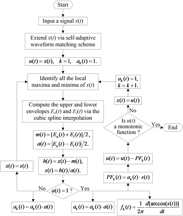
When subsections 3.2 and 3.3 are orderly combined, an improved SLMD method is formed and its flowchart is shown in Fig. 1. It is well known that the LMD algorithm has a three-layer cyclic structure, while it can be clearly seen that the improved SLMD algorithm is only with a two-layer cyclic structure, so improved SLMD is relatively simple. For convenience, improved SLMD is stilled named SLMD in the following texts.
Fig. 1Flowchart of the improved YSLMD algorithm
4. Simulation and comparative study
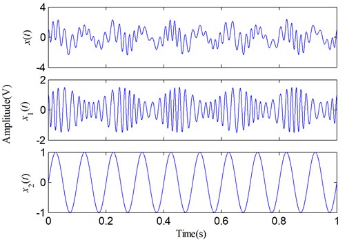
To verify the performance of the SLMD method, a comparative study on LMD and SLMD was performed via a simulative signal, which is defined as:
The waveforms of and its two components in time domain are shown in Fig. 2. There, Fig. 2 distinctly shows that has the irregularly varying frequency and amplitude, so is actually a non-stationary signal. To compare LMD and SLMD, we use them to decompose this signal, respectively, and the decomposed results are shown in Fig. 3. The obvious distinctions between the PF components and the real components cannot be easily found, but some tiny errors and differences should exist between them. In order to reveal these hidden errors and differences, a further research on the decomposed results needs to be done. Subsequently, four different aspects about the performance of LMD and SLMD are compared, and the results of the comparative study are displayed as follows.
Fig. 2A simulative signal and its two components
4.1. Iteration number and time consumption
Since the cyclic moving averaging process is replaced with the relatively simple cubic spline interpolation, the iteration number and time consumption of decomposing the given signal via SLMD should be different from those via LMD. And therefore, their respective iteration number and time consumption are compared in this part.
Fig. 3Decomposed results of the simulative signal: a) via LMD; b) via SLMD
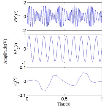
(a)
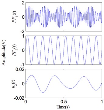
(b)
Although SLMD is different from LMD in a few computation steps, both they decompose into two PFs and a residue, and we can hardly find, only by visual observation, any obvious differences between the two decomposed results shown in Fig. 3. However, when was decomposed using LMD and SLMD, respectively, we could perceive the difference that the running time of LMD is obviously longer than that of SLMD. The actual iteration number and time consumption of decomposing via the two methods are shown in Table 1.
From Table 1, it can be seen that the iteration number of computing the PFs and the time consumption of operating the whole decomposition process of SLMD are less and shorter than those of LMD, respectively. These results indicate that SLMD actually decrease the iteration number and running time of the decomposition process, which demonstrates that the improvements of SLMD really plays an important role in improving the efficiency of computing the local mean and envelope estimate functions.
Table 1Comparison of decomposition efficiency
Algorithm | Iteration number | Time consumption (s) | |
LMD | 5 | 2 | 5.9362 |
SLMD | 3 | 1 | 2.1597 |
4.2. Errors of each PF and residue
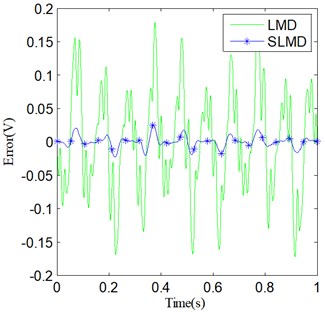
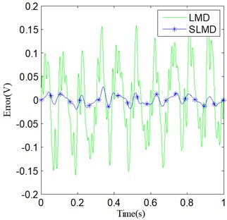
Two sets of similar decomposed results respectively shown in Figs. 3(a), (b) are compared and investigated in this part. For each , we subtract it from its corresponding real component to form a component error:
Consequently, four different error curves can be produced via Eq. (35). They are classified into two groups and shown in Fig. 4. The results obviously show that there actually are some errors between the PFs and their corresponding real components. Moreover, compared with LMD, SLMD only produces relatively small errors. In other words, each PF derived by SLMD is more accurate than that derived by LMD. As for the two residues, nothing has been done to them and they are shown in Fig. 5. It can be seen that the residue produced by SLMD is closer to a zero vector than that produced by LMD.
Fig. 4Errors of the two sets of PFs: a) e1(t); b) e2(t)
(a)
(b)
Fig. 5Two residue u2(t)
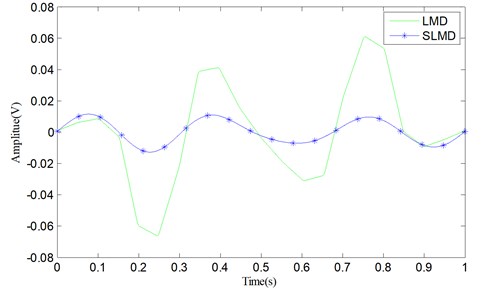
In fact, since SLMD can produce more accurate PFs than LMD and the residue is equal to the original signal subtracting the corresponding PFs, the residue resulting from SLMD should be smaller than that resulting from LMD. Table 2 shows the integrals of the absolute errors and residues produced by LMD and SLMD, respectively. Each integral value is computed by:
where represents the errors , and the residue . From Table 2, we can see that the integral values of three error functions (including the residue) resulting from SLMD are obviously smaller than those resulting from LMD. These results indicate that SLMD can more accurately decompose the non-stationary signal than LMD.
Table 2Comparison of decomposition efficiency
Algorithm | |||
LMD | 0.0644 | 0.0674 | 0.0231 |
SLMD | 0.0058 | 0.0080 | 0.0064 |
4.3. Accuracy of IF and IA
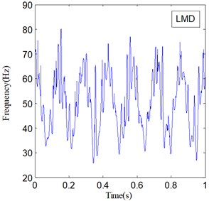
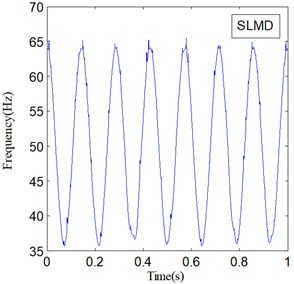
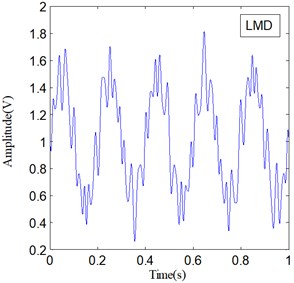
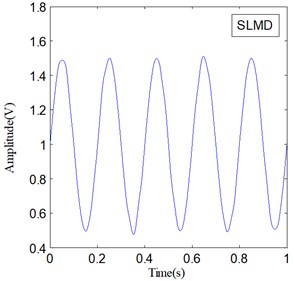
IF and IA are the important features of a non-stationary signal, and they can be obtained along with LMD and SLMD processes. Fig. 6 shows the IF of and Fig. 7 shows the IA of ; here, represents two different PF components derived by LMD and SLMD, respectively.
Fig. 6IF of PF1(t)
(a)
(b)
Fig. 7IA of PF1(t)
(a)
(b)
The two IF curves are both distorted in the whole range, but the distortions of IF in Fig. 6(a) is much severer than that in Fig. 6(b). This phenomenon illustrates that IF actually becomes more accurate because of the improvements in SLMD. Moreover, the two IA curves plotted in Fig. 7 show that the IA computed by LMD also suffers from some obvious distortions, while the IA computed by SLMD is very accurate and there is almost no distortion in the whole range. This result indicates that the SLMD method actually improves the accuracy of IA. Through comparing the two IFs and IAs, respectively, we find that SLMD actually can produce more accurate instantaneous characteristics of a non-stationary signal than LMD.
4.4. Energy error
In accordance with the basic principle of signal decomposition, any signal can be expressed as:
where is the coefficient, and is the basic function. So, the energy of can be determined by:
If is an orthogonal basis set, the energy can be written as:
On the other hand, respective PFs derived by LMD and SLMD are almost orthogonal to each other, i.e., any two different PFs satisfy the following condition [23]:
where represents the inner product operator. Therefore, each component is essentially a PF, i.e.:
Substituting Eq. (41) into Eq. (39) gives:
It should be noted that the residue is neglected in Eq. (42). Generally, the better orthogonality a group of PFs possess, the smaller the error existing in Eq. (42) becomes. In other words, the error between two sides of the approximately equal sign “” in Eq. (42) can reflect the performance of LMD and SLMD to some extent. In fact, when a non-stationary signal is decomposed by any method, the signal energy computed via the decomposed components will change more or less. Therefore, the energies of the three groups of signal sets are calculated through Eq. (42), respectively. For clarity and convenience, the energy of the original signal is denoted by , and the energies of the PFs derived by LMD and SLMD are denoted by and , respectively. The three computed energy values are shown in Table 3. From Table 3, it can be easily found that the value of is the largest and the value of is the smallest. Although and are not equal to , both they are very close to . However, the energy error between and is 0.0872, while the energy error between and is only 0.0100. The result indicates that the PFs derived by SLMD make the error in Eq. (42) smaller than those derived by LMD, which verifies that SLMD actually can produce more accurate PFs than LMD.
Table 3Comparison of the signal energies
Energy notation | Energy value |
E0 | 1.0643 |
E1 | 0.9771 |
E2 | 1.0543 |
It is clearly demonstrated through the above comparative study in four aspects that SLMD actually outperforms LMD in computational accuracy and efficiency. The improvements of SLMD play an important role in computing the local envelope and mean functions, and consequently, the derived PFs, IA and IF all become more accurate. SLMD not only reduces the running time of decomposing a signal, but also makes the instantaneous characteristics of a no-stationary signal more accurate. Therefore, SLMD indeed has a more powerful ability in processing the complicated non-stationary signal than LMD.
5. Experimental verification
Rotor-bearing system is the most important component of rotating machinery. The vibration signals acquired from it usually show the highly non-stationary characteristics, but meanwhile this kind of signal always carries abundant operating state information about rotating machinery. Therefore, analyzing the vibration signal is a very effective scheme for machine fault diagnosis and feature extraction [20]. To verify the performance of SLMD, a vibration experiment was performed on a rotor-bearing test rig with slight rub-impact fault. Fig. 8 shows a photograph of the rotor-bearing rig, and a rubbing stick marked on the graph is used to trigger the rub-impact fault. In this experiment, the rotor runs at 2800 rpm, the sampling frequency is 5000 Hz and 3000 data points are acquired for a sample signal.
Fig. 8A photograph of the experimental rotor-bearing rig
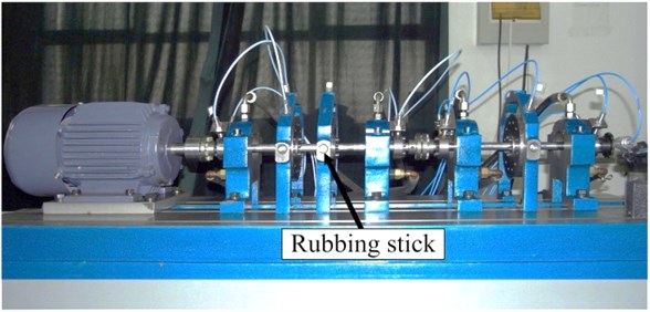
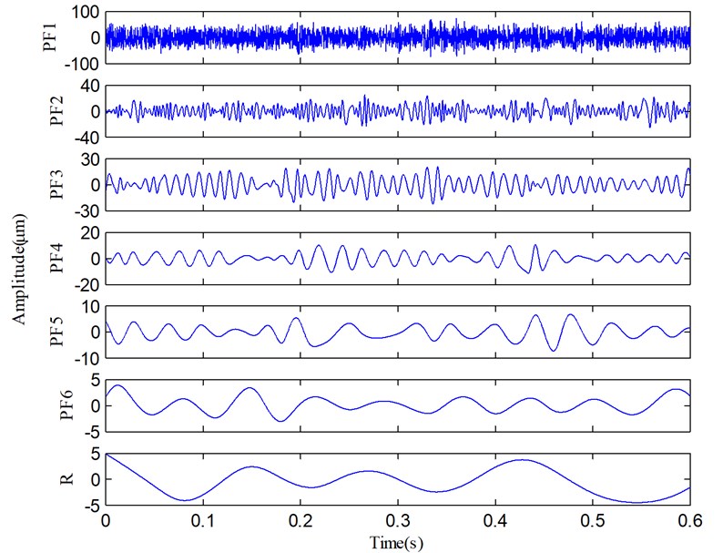
Fig. 9 shows the time domain waveform and Fourier spectrum of a sample signal. There, it can be seen that the fault vibration signal and its spectrum are very complicated. The complex spectrum indicates that the fault features can hardly be found from a complicated vibration signal only via the Fourier transform, so the signal needs to be processed via other methods. Subsequently, the SLMD method is used to process this signal, and the decomposed result is shown in Fig. 10. Obviously, the vibration signal is decomposed into six PF components from high to low frequency and a residue.
Fig. 9The sampled vibration signal and its spectrum
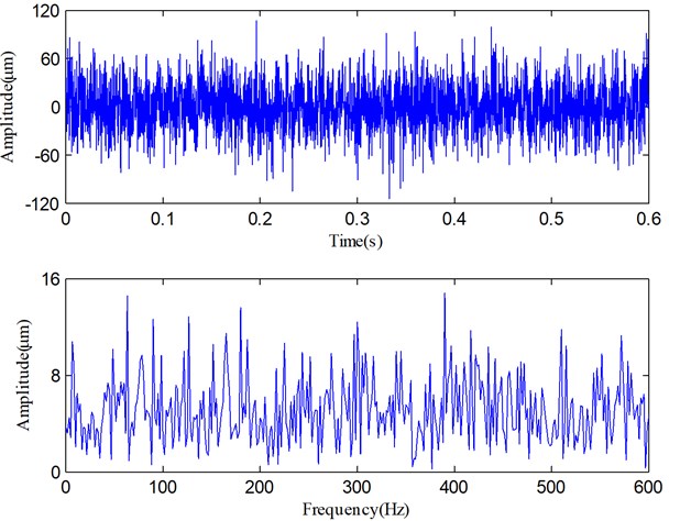
Fig. 10The decomposed results of the vibration signal via SLMD

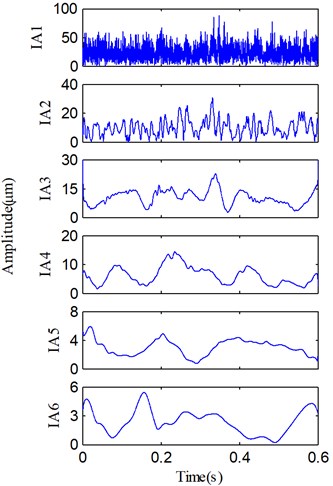
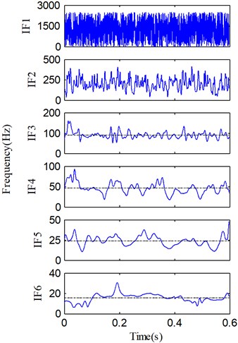
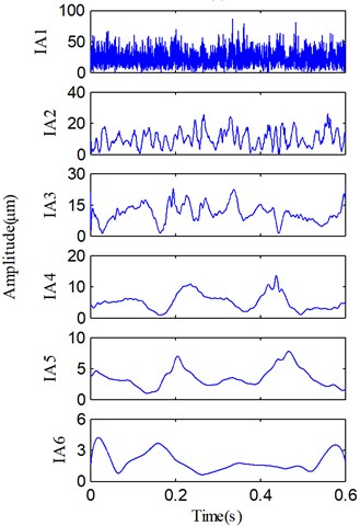
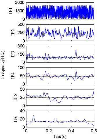
It can be found that PF1 contains the high-frequency and impulse components which should be some random and system noises. These noises heavily distort the pure vibration signal, and therefore, the waveform and spectrum shown in Fig. 9 are so complicated. Along with the decomposition process, IA and IF of each PF are also derived and shown in Fig. 11. The dynamic characteristics of the rotor can be obtained via the comprehensive analysis of the IF spectra in Fig. 11.
From Fig. 11(b), we can find that IF2 fluctuate sharply and the mean of IF2 is about 260 Hz, so PF2 is mainly the high-order vibration harmonics. Because the fault information contained in high-order harmonic components is quite limited, very few fault features can be extracted from PF2 component. However, the rest of PFs (i.e., PF3-PF6) are useful components which contain the important fault information. Although four irregularly varying IFs reveal that the rotor runs under an unsteady condition, the averages of IF3, IF5 and IF6 are equal to 93.3 Hz, 23.5 Hz and 15.2 Hz. On the other hand, the fundamental harmonic (i.e., rotating frequency) of the rotor is about 46.6 Hz (1X), so 93.3 Hz, 23.5 Hz and 15.2 Hz correspond to the second harmonic 2X, the fractional harmonics X/2 and X/3, and these harmonic components are just the rub-impact fault symptoms [9]. According to these analyses, we can easily recognize that PF3, PF4, PF5 and PF6 correspond to the 2X, 1X, X/2 and X/3, respectively. On the basis of above analyses, a purified vibration signal is reconstructed using the useful PFs (PF3-PF6) through Eq. (9). The reconstructed vibration signal and its Fourier spectrum are shown in Fig. 12.
It can be easily seen that compared with Fig. 9, Fig. 12 clearly illustrates the fundamental harmonic component (1X), the fractional and second harmonic components (X/3, X/2 and 2X). The results shown in Figs. 11 and 12 indicate that SLMD not only can obtain the instantaneous characteristics of the vibration signal, but also can successfully extract the X/3, X/2 and 2X components which are generated by the rub-impact fault.
All above diagrams and corresponding analyses can reveal that the rub-impact fault actually exists in the experimental rotor-bearing system, which proves that SLMD is suitable to process the vibration signal resulting from a rotating machine.
Fig. 11a) IA and b) IF of each PF in Fig. 10, and the average of useful IFs (dashed line)
(a)
(b)
To further validate the effectiveness of SLMD, LMD is used to decompose the same vibration signal for a comparative study. The decomposed results produced by LMD are shown in Fig. 13. Comparing the two groups of PFs plotted in Figs. 10 and 13, we can easily derive these results: 1) both SLMD and LMD can decompose the vibration signal into six PFs and a residue; and 2) each PF produced by SLMD is very similar to the homologous PF produced by LMD. However, there are some small differences between the two sets of PFs. The periodic oscillations in the PF3, PF4 and PF5 produced by SLMD are more obvious than those produced by LMD.
Fig. 12The vibration signal reconstructed with useful PFs in Fig. 10 and its spectrum
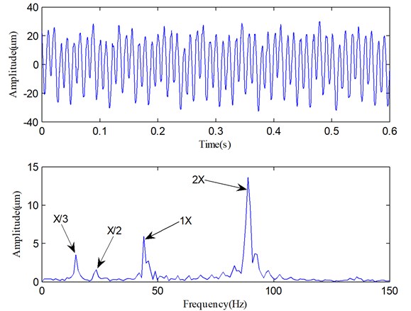
Fig. 13The decomposed results of the vibration signal via LMD.
In addition, the IAs and IFs of the all PFs derived by LMD are also illustrated in Fig. 14, respectively. Comparing Figs. 11 and 14, we can find that the IAs and IFs of the four useful PFs produced by SLMD and LMD, respectively, are obviously different. There are two reasons for this. First, due to the strong noises in the raw vibration signal, SLMD and LMD will be affected at different degrees. Second, compared with LMD, SLMD can produce relatively accurate local mean and envelope estimate functions in the process of signal decomposition. Although the two groups of IAs and IFs are different, the averages of the four IFs (dashed lines) in Fig. 11 are almost equal to those in Fig. 14. In other words, the rub-impact fault features (i.e., the second harmonic 2X, the fractional harmonics X/3 and X/2) can be correctly extracted by SLMD and LMD, respectively, but SLMD produces more accurate PFs and corresponding IFs.
Furthermore, Fig. 15 displays the reconstructed vibration signal and its Fourier spectrum as Fig. 12 shows. We can find that the characteristic frequencies of rub-impact fault (the X/3, X/2 and 2X components) in Fig. 15 are nearly as clear as that in Fig. 12, but the noise components also become relatively obvious, which makes the low-frequency characteristics not very clear. All these results indicate that SLMD and LMD produce two similar decomposed results, but SLMD can separate out more accurate PFs from the non-stationary vibration signal. Therefore, the comparative study verifies that SLMD can more accurately extract the significant fault features from the mechanical vibration signal than LMD.
And lastly, the iteration number of forming each PF component and the time consumption of decomposing the mechanical vibration signal via LMD and SLMD algorithms, respectively, are also shown in Table 4.
It can be clearly seen that in the process of decomposing the vibration signal, the iteration number of computing each PF is smaller via SLMD than via LMD; the time consumption of deriving six PFs is also much shorter via SLMD than via LMD. These results indicate that SLMD can obviously decrease the iteration number and time consumption of the decomposition process of the mechanical vibration signal, which demonstrates that cubic spline interpolation and signal extending based on self-adaptive waveform matching technique commonly promote the performance of SLMD and really play a very useful role in improving the efficiency and accuracy of SLMD. Therefore, through this experimental verification, it is proved that the improvements to LMD are quite successful and consequently results in a more effective method, SLMD, for analyzing the complicated non-stationary signals.
Fig. 14a) IA and b) IF of each PF in Fig. 13, and the average of useful IFs (dashed line)
(a)
(b)
Fig. 15The vibration signal reconstructed with useful PFs in Fig. 13 and its spectrum
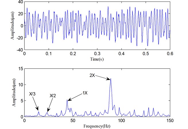
Table 4Comparison of decomposition efficiency
Algorithm | Iteration number | Time consumption (s) | |||||
LMD | 5 | 12 | 22 | 27 | 6 | 3 | 71.3 |
SLMD | 4 | 8 | 13 | 15 | 6 | 2 | 39.2 |
6. Conclusions
As a novel time-frequency analysis method for processing the non-stationary signal in recent years, LMD has been increasingly studied in machine fault diagnosis. However, LMD is not always efficient and accurate, especially for processing mechanical vibration signal. In this paper, we propose a new scheme to improve the LMD algorithm. According to the new scheme, cubic spline interpolation and self-adaptive waveform matching techniques are combined and integrated into LMD to form an improved SLMD method, which can decrease the time consumption and improve the computational accuracy. Then, the comparative studies through a simulative signal and an experimental vibration signal are presented, respectively. Simulative results show that SLMD actually outperforms LMD in computational efficiency and accuracy; experimental results show that fault features of a rotating machine with slight rub-impact can be more accurately and efficiently extracted from the vibration signal via SLMD. These results prove that the improvements to LMD are very successful and SLMD is actually quite suitable for non-stationary signal analysis and vibration signal analysis of rotating machinery.
References
-
Feng Z. P., Zuo M. J. Vibration signal models for fault diagnosis of planetary gearboxes. Journal of Sound and Vibration, Vol. 331, Issue 22, 2012, p. 4919-4939.
-
Lee B. J., Kim K. H., Ku B., Jang J. S., Kim J. Y. Prediction of body mass index status from voice signals based on machine learning for automated medical applications. Artificial Intelligence in Medicine, Vol. 58, Issue 1, 2013, p. 51-61.
-
Roveri N., Carcaterra A. Damage detection in structures under traveling loads by Hilbert-Huang transform. Mechanical Systems and Signal Processing, Vol. 28, 2012, p. 128-144.
-
Pai P. F. Time-frequency analysis for parametric and non-parametric identification of nonlinear dynamical systems. Mechanical Systems and Signal Processing, Vol. 36, Issue 2, 2013, p. 332-353.
-
Qi K. Y., He Z. J., Zi Y. Y. Cosine window-based boundary processing method for EMD and its application in rubbing fault diagnosis. Mechanical Systems and Signal Processing, Vol. 21, Issue 7, 2007, p. 2750-2760.
-
Feng Z. P., Liang M., Chu F. L. Recent advances in time–frequency analysis methods for machinery fault diagnosis: A review with application examples. Mechanical Systems and Signal Processing, Vol. 38, Issue 1, 2013, p. 165-205.
-
Huang N. E., Shen Z., Long S. R., Wu M. C., Shih H. H., Zheng Q., Yen N. C., Tung C. C., Liu H. H. The empirical mode decomposition and the Hilbert spectrum for nonlinear and non-stationary time series analysis. Proceedings of the Royal Society of London, Series A, Vol. 454, 1998, p. 903-995.
-
Smith J. S. The local mean decomposition and its application to EEG perception data. Journal of the Royal Society Interface, Vol. 2, Issue 5, 2005, p. 443-454.
-
Wang Y. X., He Z. J., Zi Y. Y. A comparative study on the local mean decomposition and empirical mode decomposition and their applications to rotating machinery health diagnosis. ASME Journal of Vibration and Acoustics, Vol. 132, Issue 2, 2010, p. 0210101.
-
Chen B. J., He Z. J., Chen X. F., Cao H. R., Cai G. G., Zi Y. Y. A demodulating approach based on local mean decomposition and its applications in mechanical fault diagnosis. Measurement Science and Technology, Vol. 22, Issue 5, 2011, p. 055704.
-
Cheng J. S., Zhang K., Yang Y. An order tracking technique for the gear fault diagnosis using local mean decomposition method. Mechanism and Machine Theory, Vol. 55, Issue 9, 2012, p. 67-76.
-
Yang Y., Cheng J. S., Zhang K. An ensemble local means decomposition method and its application to local rub-impact fault diagnosis of the rotor systems. Measurement, Vol. 45, Issue 3, 2012, p. 561-570.
-
Wang Y. X., He Z. J., Zi Y. Y. A demodulation method based on improved local mean decomposition and its application in rub-impact fault diagnosis. Measurement Science and Technology, Vol. 20, Issue 2, 2009, p. 025704.
-
Cheng J. S., Yang Y., Yang Y. A rotating machinery fault diagnosis method based on local mean decomposition. Digital Signal Processing, Vol. 22, Issue 2, 2012, p. 356-366.
-
Wang Y. X., He Z. J., Xiang J. W., Zi Y. Y. Application of local mean decomposition to the surveillance and diagnostics of low-speed helical gearbox. Mechanism and Machine Theory, Vol. 47, 2012, p. 62-73.
-
Liu W. Y., Zhang W. H., Han J. G., Wang G. F. A new wind turbine fault diagnosis method based on the local mean decomposition. Renewable Energy, Vol. 48, 2012, p. 411-415.
-
Zhang Y., Qin Y., Xing Z. Y., Jia L. M., Cheng X. Q. Roller bearing safety region estimation and state identification based on LMD-PCA-LSSVM. Measurement, Vol. 46, Issue 3, 2013, p. 1315-1324.
-
He Z., Shen Y., Wang Q. Boundary extension for Hilbert–Huang transform inspired by gray prediction model. Signal Processing, Vol. 92, Issue 3, 2012, p. 685-697.
-
Qin Y. Multicomponent AM–FM demodulation based on energy separation and adaptive filtering. Mechanical Systems and Signal Processing, Vol. 38, Issue 2, 2013, p. 440-459.
-
Patel T. H., Darpe A. K. Coupled bending-torsional vibration analysis of rotor with rub and crack. Journal of Sound and Vibration, Vol. 326, Issue 3-5, 2009, p. 740-752.
-
Shao C. X., Wang J., Fan J. F., Yang M., Wang Z. C. A Self-adaptive method dealing with the end issue of EMD. Acta Electronica Sinica, Vol. 35, Issue 10, 2007, p. 1944-1948.
-
Hu A. J., An L. S., Tang G. J. New process method for end effects of Hilbert-Huang Transform. Journal of Mechanical Engineering, Vol. 44, Issue 4, 2008, p. 154-158.
-
Zhang K., Cheng J. S., Yang Y. Product function criterion in local mean decomposition method. Journal of Vibration and Shock, Vol. 30, Issue 9, 2011, p. 84-88.
About this article

This work is supported by the National Natural Science Foundation of China (Nos. 50875118 and 51165019) and Cultivation Program for Excellent Doctoral Dissertation of Lanzhou University of Technology (No. 201102).
