Damage detection by the curvature of POMs extracted from measured FRF data

1. Introduction

Structural health monitoring has been receiving a growing amount of interest from researchers in diverse engineering fields, such as aerospace, mechanical and civil engineering. Structural damage detection techniques involve the process of detecting, locating, and quantifying damage in a structure by observing changes in the structure response. Many non-destructive methods for improved serviceability and damage detection of structures have been developed with the advent of new measuring systems. During the past several decades, a significant amount of research has been conducted in the area of structural damage detection [1, 2]. Most of the damage detection methods require the baseline data to compare with the measured data in the damaged state.

The proper orthogonal decomposition (POD) is a multi-variate statistical method that aims at obtaining a compact representation of the data. The POD extracts a basis to decompose the data so that the projection of the data contains as much energy as possible. The POD known as the Karhunen-Loeve Decomposition (KLD) recently revealed a useful tool for the analysis of mechanical dynamical systems. The POD reduces a large number of interdependent variables to a small number of uncorrelated variables and provides relevant structure hidden in the data. The POD involves two steps of extraction of POMs, and the projection of basis functions to obtain a low-dimensional dynamic model. The POMs constitute a set of optimal basis functions with respect to the energy content of the signal. The POM obtained from the PODs effectively extracts the principal component of a large DOF system or complex physical phenomena. The POD is also used in detecting the number of signals in a multichannel time-series [3], capturing the modes of a reaction-diffusion chemical process [4] and describing quantitative changes in spatial complexity during extended episodes of ventricular fibrillation [5]. The method can be applied in obtaining reduced-order models of unsteady viscous flows [6], forecasting in meteorology [7] and classifying speech data [8].

The POD method can be widely used in detecting structural damage. De Boe and Golinval [9] presented a damage detection method using PCA of a sensor array. The method does not require the structural excitation or a structural model. Correlating the dynamic response of a vehicle with changes in track and support geometry, Feldmann et al. [10] provided a method to constantly monitor track condition. Based on the POD technique, Shane and Jha [11] proposed a damage detection method of structural health monitoring. Lanata and Grosso [12] presented a damage detection method using the POD for a temporal and spatial correlation analysis between the structural responses measured at different sensor locations. Based on the use of singular value decomposition (SVD), Ruotolo and Surace [13] provided a damage detection method for detecting damage in structures at an early stage with dynamic characteristics that may change during the lifetime without mathematical models of the analyzed structure.

Taking the POMs that contain the greatest amount of energy in the signal, Lenaerts et al. [14] presented a time domain method for the identification of non-linear parameters of a model. Galvanetto and Violaris [15] used the POD methods to provide the characteristic shape of the deformed structure during the steady-state dynamics and presented the damage detection method based on the change in the shape.

It has been reported [16] that FRF data provide more information than modal data, as the latter are extracted from a very limited frequency range related to resonance. The FRF curvature method and mode shape curvature method require the baseline data in the intact state. Sampaio et al. [17] provided a damage detection method using the FRF curvature method. It is the damage detection method by summing up the absolute difference between the FRF curvatures of the damaged and undamaged structure within a given frequency range. They compared with the mode shape curvature method and the damage index method, which require the baseline data.

The damage should be detected only by the measured data at the damaged state because the initial data are not available. Ratcliffe [18] presented a damage identification method in a beam without any information on its intact state. The method calculated a difference function between the cubic and Laplacian, and detected localized damage to a structure. Ratcliffe and Bagaria [19] presented the Gapped-Smoothing Method (GSM) to detect damage from the distribution of curvature mode shapes. Lee and Eun [20] presented a method to detect damage utilizing only the measured strain data collected from a damage-expected beam structure without intact baseline data.

This study provides a damage detection method to recognize structural defect based on the curvature of POMs extracted from measured FRF response data. The merit of the proposed method doesn’t require the input data and the intact baseline data of a dynamic system. It is demonstrated that the proposed method and Ratcliffe’s method should be sensitive to the FRF data corresponding to frequency range to be considered. Both methods should be sensitive to the external noise included in the measured FRF data. Despite such noise the effectiveness of this method is illustrated in a numerical application and a beam test. It is shown in the applications that the proposed method is less sensitive to external noise than the Ratcliffe’s method and the FRF curvature method cannot be utilized in detecting damage without the baseline data.

2. FRF of dynamic system

The dynamic response of a structure can be expressed in the time and frequency domains. This work begins with the derivation of FRF responses measured in the frequency domain. The dynamic behavior of a structure that is assumed to be linear and approximately discretized for $n$ DOFs can be described by the equations of motion as:

where $\mathbf{M}$ and $\mathbf{K}$ denote the $n\times n$ analytical mass and stiffness matrices, $\mathbf{u}$ denotes the $n\times 1$ displacement vector, $\mathbf{C}\in R^{n\times n}$ is the damping matrix, and $\mathbf{f}\left(t\right)$ is the $n\times 1$ excitation vector.

It is important to establish a relationship between FRF and modal parameters for successful modal testing. Inserting $\mathbf{u}=\mathbf{U}{e}^{j\mathrm{\Omega }t}$ and $\mathbf{f}=\mathbf{F}{e}^{j\mathrm{\Omega }t}$ into Eq. (1) and expressing it in the frequency domain, it follows that:

where $\mathrm{\Omega }$ denotes the excitation frequency, $\mathbf{F}$ is an external force vector with an element being unit and all other elements zeros in the frequency domain, and $j=\sqrt{-1}$. And $\mathbf{U}\left(\mathrm{\Omega }\right)$ is the displacement response amplitude vector in the frequency domain. Using the impedance-type matrix of the structure $\mathbf{B}\left(\mathrm{\Omega }\right)$, the equation of motion for the initial structure in the frequency domain is expressed by:

where $\mathbf{B}\left(\mathrm{\Omega }\right)=(\mathbf{K}-{\mathrm{\Omega }}^2\mathbf{M}+j\mathrm{\Omega }\mathbf{C})$.

Using the FRF matrix, the response of the structure, described by $\mathbf{U}\left(\mathrm{\Omega }\right)$, to an external excitation, described by $\mathbf{F}\left(\mathrm{\Omega }\right)$, is given by:

where $\mathbf{H}\left(\mathrm{\Omega }\right)={\mathbf{B}}^{-1}\left(\mathrm{\Omega }\right)={(\mathbf{K}-{\mathrm{\Omega }}^2\mathbf{M}+j\mathrm{\Omega }\mathbf{C})}^{-1}$ is the FRF matrix of the structure, whose elements can be the receptances.

The elements in the FRF matrix are derived as follows. Transforming Eq. (2) into the frequency domain leads to:

where ${\omega }_i$ and ${\xi }_i$ denote circular natural frequency and damping ratio corresponding to the $i$th mode, respectively. By applying modal transformation, the real eigenvalues and eigenvectors lead to the representation of the FRF matrix for an excitation frequency $\mathrm{\Omega }$:

where ${\mathbf{\phi }}_i$ is the $i$th mode shape vector of the dynamic system. For the case of a displacement response at station $p$ and a disturbing force at station $q$, the numerical frequency response can be constructed as:

where ${\varphi }_{i,p}$ denotes the $p$th element of the vector ${\varphi }_i$. From Eq. (7), the FRF matrix should be symmetric. If a unit impulse force acts at a fixed position $l\text{,}$ we obtain ${\mathbf{H}}_{k,l}={\mathbf{U}}_l={\left[\begin{array}{cccc}{H}_{1,l}& H_{2,l}& \cdots & H_{n,l}\end{array}\right]}^T$ and ${\mathbf{H}}_{l,k}={\mathbf{U}}_l^T=\left[\begin{array}{cccc}{H}_{l,1}& H_{l,2}& \cdots & H_{l,n}\end{array}\right]$. A set of FRF response data are obtained within a given frequency range but it is unnecessary to transform the FRF data within all frequency ranges to the POMs. The FRF data within an arbitrary frequency range can lead to unwanted POMs so that they cannot be used in detecting damage. Thus, this work investigates the POM curvature according to frequency range for finding the prescribed damage.

3. Curvature of POMs

The POD extracts feature by revealing relevant, but unexpected, structure hidden in the data. The POD is used to derive a reduced-order model for non-linear initial value problems. Assume that measurement data are expressed by a finite number of points in space and frequency. Expressing a set of FRF response data as $\mathbf{U}$, suppose that $m$ linear snapshots of the response $U_i$ of size $n$ are obtained by response measurements written as:

where the superscript $\left(j\right)$ represents the FRF frequency response data at the $j$th frequency ${\mathrm{\Omega }}_j$, $n$ denotes the number of measurement positions of the structure and $m$ is the total number of frequency observations.

The POD of this discrete field entails solving the eigenvalue problem. Let $m\times m$ matrix $\tilde{\mathbf{C}}$ define as:

Solving the eigenvalue problem of Eq. (9) at the core of the POD method, it satisfies:

where the eigenvalues are arranged as:

where the eigenvalues ${\lambda }_k$ are the proper orthogonal values (POVs) and each eigenvector ${\mathbf{\phi }}_k$ of the extreme value problem is associated with a POV ${\lambda }_k$. ${\mathbf{\phi }}_1$ represents the eigenvector corresponding to the largest eigenvalue ${\lambda }_1$.

The POMs may be used as a basis for the decomposition of $\mathbf{U}$. The POM associated with the greatest POV is the optimal vector. If the eigenvalues are normalized, they represent the relative energy captured by the corresponding POM. The eigenvalue reflects relative kinetic energy associated with the corresponding mode. The energy is defined as the sum of the POVs. The POMs are written as:

The POMs are arranged as:

The structural health state can be predicted by evaluating the POMs in Eq. (13). Recognizing that the structural beam exhibits the flexural behavior, this work considers the curvature of POMs. Damage introduced into the flexural beam to be modeled as finite elements leads to local changes in the shape of POM curvature obtained by POMs. The curvature at each location $i$ on the structure, ${{\mathbf{\psi }}_j^i}^{\mathrm{\text{'}}\mathrm{\text{'}}}$ is numerically obtained by a central difference approximation:

where ${{\mathbf{\psi }}_j^i}^{\text{'}\text{'}}$ is the second derivatives at the $j$th node of the $i$th POM and the $h$ is the distance between two successive nodes. This work utilizes the curvature relation of Eq. (14) from POMs to detect damage instead of displacement mode shape or FRF data.

4. Applications

4.1. Numerical experiment

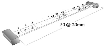
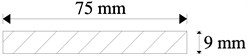
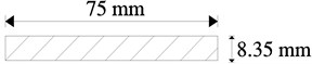
The validity of the proposed POM curvature method is illustrated in a numerical experiment of a fixed-end beam shown in Fig. 1. The numerical results are compared with those obtained by other methods. The nodal points and the members are numbered as shown in the figure. Assuming Bernoulli-Euler plane beam element, the beam finite elements are obtained by subdividing beam members longitudinally. Each node has two dofs of transverse displacement and slope. A beam of 1 m length was modeled using 50 beam elements. The beam has an elastic modulus of 2.0×10⁵ MPa and a unit mass of 5000 kg/m³. Its gross cross section is 75 mm×9 mm and its damage section is established as 20 % loss on the initial second moment of inertia.

Fig. 1Finite element model for a fixed-end beam: (a) a fixed-end beam, (b) undamaged cross section, (c) damaged cross section

(a)

(b)

(c)

This numerical application considers the damage detection of a fixed-end beam with multiple damages. It is expected that there would be some deviation due to the noise in measurement data. For this numerical application, the noise is simulated by adding a series of random numbers on calculated FRF response data. The FRF response data are measured by the roving of accelerometer under the excitation of the impact hammer at a reference point or by the accelerometer at a reference with the roving of the hammer. The FRF response $H_{i,j}$ indicates a displacement response at station $i$ and a disturbing force at station $j$. Thus, the measured FRF response $H_{i,j}^m$ can be calculated of the simulated noise-free FRF data $H_{i,j}^0$ as:

15

$H_{i,j}^m=H_{i,j}^0\left(1+\alpha {\sigma }_{i,j}\right),$

where $\alpha$ denotes the relative magnitude of the error and ${\sigma }_{i,j}$ is a random number variant in the range $[-1,1]$. Based on these variables and an assumption of 3 % noise magnitude, this numerical application considers a damaged beam with multiple damages at elements 22 and 37.

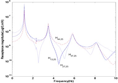
Figure 2 represents the FRF curves of the fixed-end beam with multiple damages. In the plots, $H_{i,25}$ ($i=$13, 27, 37, 44) denotes the dynamic response at nodes 13, 27, 37 and 44 due to a unit impulse at node 25, respectively. The $y$-axis in the plot represents the logarithmic scale of the receptance magnitude in the range of 0.01–10 Hz with the step of 0.02 Hz. It is shown that the first and second resonances locate near the frequencies of 1.2 Hz and 2.3 Hz, respectively.

Fig. 2FRF curve in the range of 0.01–10 Hz contaminated by 3 % noise

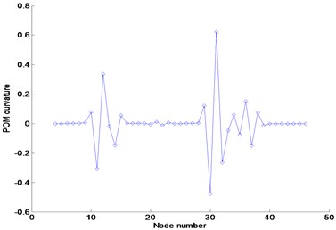
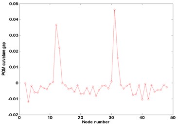
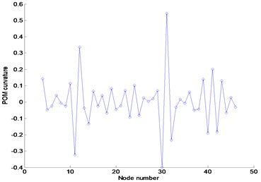
The FRFs and POMs are extracted from the data within frequency range to be considered. We utilized the FRF data $H_{i,1}^j$ to collect from two different range of 1.1–1.2 Hz and 3–3.1 Hz in the neighborhood of the first and third resonance frequencies, respectively. Here, the superscript $j$ denotes the number of frequency observations and the subscript $i$ indicates the measurement position of the dynamic response due to a unit impulse at node 1 corresponding to each frequency. Figure 3 represents the numerical results obtained by FRF curvature method and Ratcliffe’s method, and the proposed method. Figure 3(a) represents the noise-free FRF curvature in the frequency range of 1.1–1.2 Hz. The curvature was estimated by a central difference method. The FRF curvature method properly detects the damage by investigating the absolute difference between the FRF curvature of the undamaged and damaged structure. The damage exists at the location to represent the abrupt variation of FRF curvature. The plot indicates that the FRF curvature can certainly detect the damage in the noise-free case using the FRFs only in the damaged state without the initial baseline data. We compared the proposed method with the Ratcliffe’s method introduced in the Appendix which doesn’t require the baseline data. Figure 3(b) represents the POM curvature gap using POMs corresponding to the first POV instead of mode shape data based on the Ratcliffe’s method. It is found that the Ratcliffe’s method properly indicates the damage location. Figure 3(c) exhibits the POM curvature plots corresponding to the first POV. The POM curvature at the damage location displays more abrupt change than other locations. The change in the POM curvature indicates the abrupt variation in energy due to the damage.

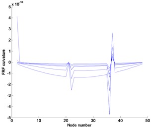
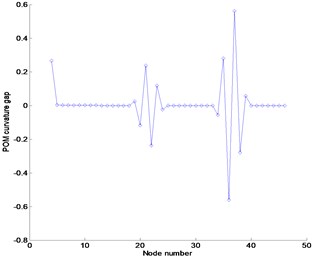
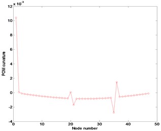
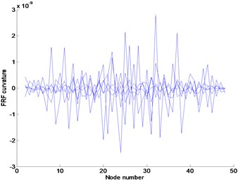
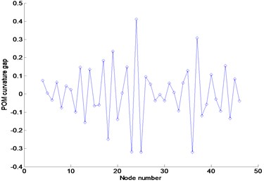
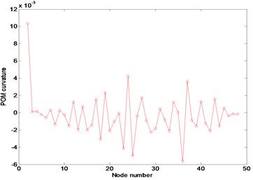
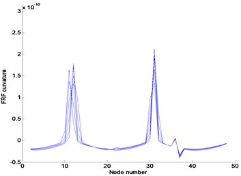
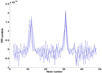
The responses considering external noise are displayed in Fig. 4. Ten numerical experiments were repeated for describing various noise conditions. Figure 4(a) represents the FRF curvature at the frequency 1.1 Hz using ten sets of contaminated FRF data. It reveals that the FRF curvature method is very sensitive to noise. As a result, the method cannot be used in detecting damage. The POMs were extracted from all FRF data of ten numerical experiments in the frequency range of 1.1–1.2 Hz. Figures 4(b) and (c) exhibit the POM curvature gap by the Ratcliffe’s method and the POM curvature provided in this study. Both methods take irregular shapes due to the noise and it seems that they are sensitive to external noise. They exhibit similar plots and reveal that the damage location is properly detected.

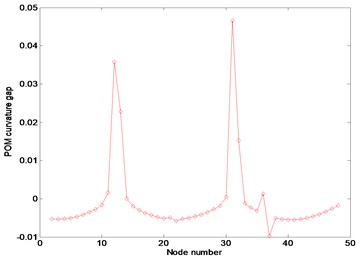
Figures 5 and 6 represent the results using the FRF data without and with external noise in the frequency range of 3–3.1 Hz, respectively. The plots exhibit the abrupt changes of responses at various locations such that the damage cannot be detected. They indicate that the damage exists nearby nodes 12 and 32 rather than the accurate positions regardless of the existence of external noise. Based on the plots, it can be recognized that the proposed method and Ratcliffe’s method are deeply affected depending on the selection range of FRF data. The selection of the FRF data beyond the first resonance frequency makes the damage detection very difficult. It can be concluded that the selection of the FRF data within the first resonance frequency range is necessary for proper damage detection rather than beyond the first resonance frequency.

Fig. 3Numerical results at noise-free case in the frequency range of 1.1–1.2 Hz: (a) FRF curvature at frequency 1.1 Hz, (b) Ratcliffe’s method, (c) POM curvature corresponding to the first POV

(a)

(b)

(c)

Fig. 4Numerical results using FRFs contaminated by 3 % noise in the frequency range of 1.1–1.2 Hz: (a) FRF curvature at frequency 1.1 Hz, (b) Ratcliffe’s method, (c) POM curvature corresponding to the first POV

(a)

(b)

(c)

Fig. 5Numerical results at noise-free case in the frequency range of 3–3.1 Hz: (a) FRF curvature at frequency 1.1 Hz, (b) Ratcliffe’s method, (c) POM curvature corresponding to the first POV

(a)

(b)

(c)

Fig. 6Numerical results using FRFs contaminated by 3 % noise in the frequency range of 3–3.1 Hz: (a) FRF curvature at frequency 1.1 Hz, (b) Ratcliffe’s method, (c) POM curvature corresponding to the first POV

(a)

(b)

(c)

4.2. Beam test

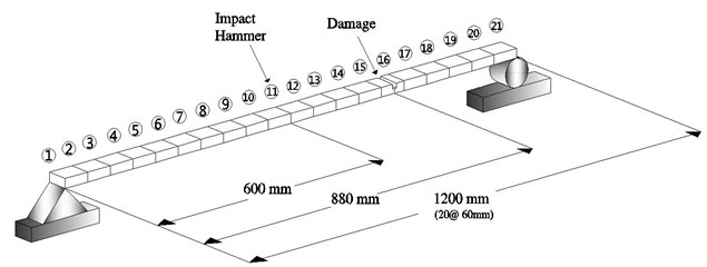
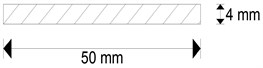
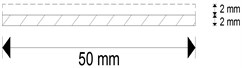
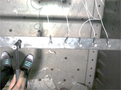
An experimental work was performed for detecting damage of a simply supported beam in Fig. 7. The test was carried out to evaluate and compare the applicability of the Ratcliffe’s method and the proposed method in the actual beam. The gross cross-section of the beam is 50 mm×4 mm and its length is 1200 mm. The damage locates at the distance of 880 mm from the left support. The damaged cross-section was established as 50 mm×2 mm. The experiment was conducted with the roving of accelerometers. The impact and 21 measurement points are numbered as shown in the figure. As shown in Fig. 8, the hammer has been impacted at a single reference point to excite the beam, whereas five uniaxial accelerometers roved around. The experiment was conducted using DYTRAN model 3055B1 uniaxial accelerometers, along with a miniature transducer hammer Brüel and Kjaer model 8204 for the excitation of the system. The data acquisition system was a DEWETRON model DEWE-43. The measured data by DEWETRON are collected as FRF which is defined as the ratio of the response of a system to its excitation force.

Fig. 7Damage and measurement locations of test beam

(a)

(b)

(c)

Fig. 8Set up of measurement sensors and impact hammer

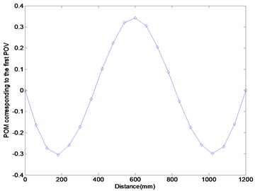
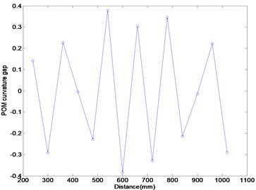
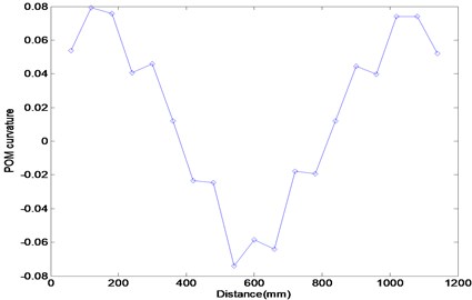
Ten experiments on the same beam were repeated for describing various noises. Figure 9 represents the FRF curves at nodes 6–10 due to an impulse at node 11. It is displayed that the first and third resonance frequencies locate in the neighborhood of 7 Hz and 56 Hz, respectively. As performed in the previous numerical experiment, the FRF data in the first and third resonance frequency range were collected to extract the corresponding POMs and the results were compared. Figure 10(a) represents the POM corresponding to the first POV extracted from the collected FRF data in the first resonance frequency range. The plot is similar to the first mode shape curve of the damaged beam. The POM data are transformed to the curvature to utilize in detecting damage. Figures 10(b) and (c) compare the Ratcliffe’s method and the proposed method. It is observed that the damage locates at the abrupt variation of the curve and both methods are sensitive to the measurement noise. The Ratcliffe’s method indicates the damage around 950 mm from the left end beyond the actual damage position. It is found that the proposed method detects more accurate damage location rather than the Ratcliffe’s method. The comparison illustrates that the proposed method is less sensitive to the noise than the Ratcliffe’s method.

Fig. 9FRF curves at nodes 6–10 due to an impulse at node 11

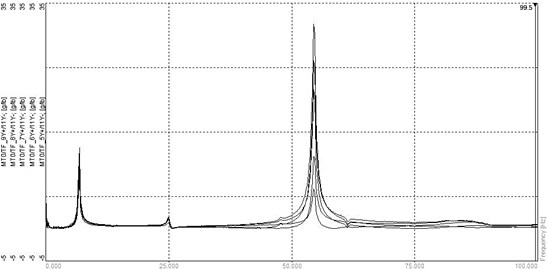
Fig. 10Numerical results using FRFs in the first resonance frequency range: (a) POM curve corresponding to the first POV, (b) Ratcliffe’s method, (c) this study

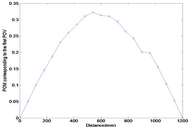
(a)

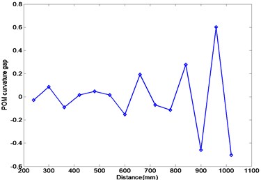
(b)

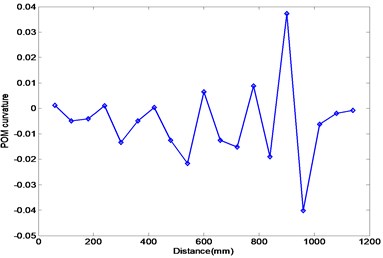
(c)

Figure 11 represents the experimental results using the FRF data in the third resonance frequency range. Figure 11(a) exhibits the POM curve corresponding to the first POV, and it is similar to the third mode shape of the damaged beam. It indicates that the POM curve to extract from the measured FRF data is similar to the mode shape of the damaged beam. Figures 11(b) and (c) provide the results calculated by the Ratcliffe’s method and this study. It is investigated that both methods do not provide the information on the damage detection and only the first POM using the FRF data in the first resonance frequency range can be utilized in detecting damage.

Both methods lead to the similar results under the numerically simulated noise and are affected depending on the FRF data region to be selected for the damage detection. The proposed method detects more accurate damage location than the Ratcliffe’s method in the actual test when the first POM using the FRF data in the first resonance frequency range is utilized. It can be concluded that the proposed method can be effectively utilized in detecting the damage of the beam without the initial baseline data under the external noise.

Fig. 11Numerical results using FRFs in the third resonance frequency range: (a) POM curve corresponding to the first POV, (b) Ratcliffe’s method, (c) this study

(a)

(b)

(c)

5. Conclusions

This work presented the POM curvature method for damage detection of a beam structure. The method does not require the input information and the baseline data of the initial undamaged structure. It used POMs to transform numerically simulated FRF data. It was shown that the damage can be detected by the POM curvature distribution from a central difference approximation of the POM corresponding to the first POV. It was recognized from the numerical and experimental application that the proposed method is a little less sensitive to the noise than Ratcliffe’s method. Also, both methods are affected depending on the FRF data region selected for the damage detection. Therefore, if the baseline data of undamaged structure do not exist and the noise is included in the measured data, the proposed method can be effectively utilized in detecting damage based on the POM curvature using the FRF data in the first resonance frequency range.