Intelligent fault classification of rolling bearings using neural network and discrete wavelet transform

1. Introduction

Automatic fault diagnosis techniques have been developed to prevent human and financial losses and increase productivity and production rate [1]. Rolling element bearings are one of the most important and most used parts in rotating machineries and are the focus of nondestructive test for fault diagnosis. Rolling element bearings faults can be due to different factors such as: wrong design or wrong mount, improper lubrication, plastic deformation etc. The most common fault is due to material fatigue after some definitive work period. This phenomena starts with developing small cracks on the surface of bearing elements. Due to fluctuating loads, these cracks grow to the surface and cause the piercing or fracture of the surface. In this research crack fault in inner race, outer race, and balls are considered.

There are many techniques which can be used for bearing fault diagnosis. The need for automation, optimization, and cost reduction were the motivation for using artificial inteligence in this regards. Fuzzy logic [2], Genetic Algorithm [3] and Artificial Neural Networks (ANN) [4] are among soft computing techniques which are used in fault diagnosing. ANN is a concept which is developed and inspired from biological and neural system of human. NN has attained a crucial role in technical and engineering applications as a nonlinear dynamical system for problem solving [5]. Like human brain NN needs training for problem-solving. Since learning needs a high amount of data, selection of feature vector is a key parameter in designing an efficient NN. Feature vector as the input to the network, represents the most important aspect of the problem for identification and classification of different patterns. One of the best inputs to the network is vibration signals, which is used widely in fault diagnosis of rotating machineries. Vibration signals are usually contaminated with noise. One of the techniques to denoise these signals is application of wavelet analysis. In the early 1990s Ledoc used wavelet analysis [6].

Wang and Mcfaden used wavelet for gearbox vibration analysis and found out that wavelet analysis is suitable to detect faults in its earliest stages of its development [7].

Mamo and Dias used both wavelet and Fourier transforms for feature extractions for fault detection of a power system. They found out that wavelet analysis outperforms Fourier analysis [8].

Tse and Peng used wavelet and envelope analysis for roller bearings and showed that they are better in terms of time of computations [9]. The published papers in this field show high efficiency for fault detection and show its superiority over other techniques. In 2003 a research has been carried out by Samantha and his colleagues. In this research a comparison between neural network and Support Vector Machine (SVM) had been done and was shown that both NN and SVM has 100 % efficiency in the feature extraction from vibration signals of a faulty gearbox [3].

In 2008 Rao et al. used neural network to find faults in a centrifugal pump. Two kinds of NN, one feedforward with back propagation algorithm and one with Adaptive Resonance Algorithm (ARA) were used. This research showed that adaptive resonance algorithm were more efficient than the other one [10].

In 2009 a research has been done by N. Saravan et al. In their work preprocessing of a signal by packet wavelet transform and processing with SVM and NN had been carried out. Characteristic vectors have been found by Morlet wavelet transform and are used as inputs to NN and SVM. SVM showed better results than NN in classifying faults [11].

In the current research NN has been used as fault classifier. This research divides into three sections:

Data acquisition from different bearings including bearing with the outer race, inner race and ball faults as well as a healthy bearing.

Preprocessing of the data which are vibration signals using discrete wavelet transform and obtaining a proper feature vector.

Design of NN for fault classification with high efficiency.

2. Experimental data acquisition

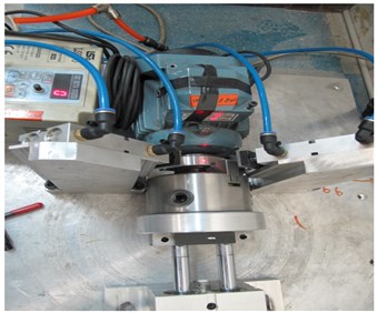
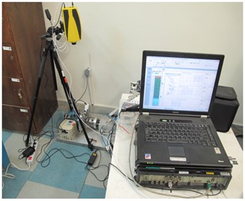
Figure 1 show the setup used in data acquisition. Our data is in the form of vibration velocity signals. Our experimental equipment constitute of the following components:

1) An electric motor with 0.5 hp.

2) A fixture for connecting electric motor to shaft with Bearing.

3) A load mechanism which puts force on the shaft.

4) Pulse 4 channel data acquisition system manufactured by B&K Company.

5) LS 600 motor speed control.

6) Laser vibration measuring system model VII-1000-D manufactured by Omron Company.

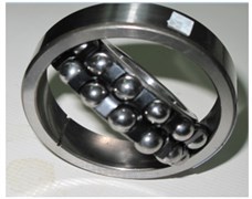
7) Double row bearings model 1206 K from Nachi Company.

Fig. 1Bearing test set up

a)

b)

The pulse multi-channel data acquisition system has four input channels and two output channels. By connecting one of its input channels to laser vibrometer, velocity vibration signals are recorded. For simulation of working condition of the bearing to be more realistic, the bearings on the test are subjected to load by a load mechanism shown in Fig. 1. The loading mechanism consists of a pneumatic actuator capable of inserting 18 Kg load on bearing. The bearings used in this test are double row bearing model 1206 K, with the spec given in Table 1.

The bearing component fault frequencies at 1800 rpm are given in Table 2.

The bearing faults frequencies are given by the following equations [12]:

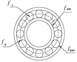
where $f_s$ is the shaft rotational frequency, $f_c$ is the cage rotational frequency, $f_{BPI}$ is the inner race frequency, $f_{BPO}$ is the outer race frequency. Also $D_b$ is ball diameter, $D_c$ is the cage diameter (the distance from the center of the one ball to the center of the opposite ball). $Z$ is the number of balls and $\theta$ is the contact angle of the balls with the race. Number of balls is 14 and $\theta$ is zero degree.

Figure 2 shows the schematic of the bearing.

Fig. 2Schematic of the bearing

Specific faults are made deliberately on the races. A groove with the depth of 3 mm and the width of 2 mm is made on the entire width of the outer race. In the second bearing a groove with the depth of 3 mm and width of 2 mm is made on the inner race. For making a fault on the balls, since usually a group of balls get faulty at the same time, some holes are developed simultaneously on four adjacent balls, as shown in Fig. 3.

Fig. 3Ball bearing with: a) outer race defect, b) inner race defect, c) ball fault

a)

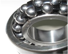
b)

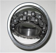
c)

Vibration signals from the rotating shaft with 1800 RPM and sampling frequency of 16 kHz are gathered for the period of 2 min with constant load. It should be noted that during the test the outer race of the bearing was fixed and rotation is applied to the inner race. Due to high amount of data signals, the signals were divided to 12 samples each having time period of 10 seconds, and the resulting signals were used. A sample of acquired signals is shown in Fig. 4.

Fig. 4Vibration signal of bearing tested at 1800 rpm: a) inner race defect, b) outer race defect, c) ball fault, d) healthy bearing

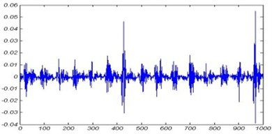
a)

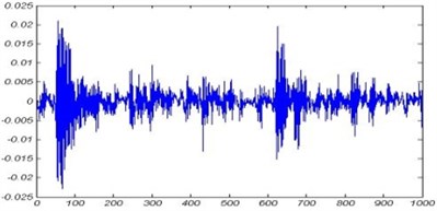
b)

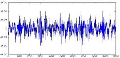
c)

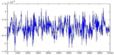
d)

3. Preprocessing of vibration signals

Wavelet transform which is an analysis technique in time frequency domain has the ability to bring out information out of a signal which has distinguished it from other analysis techniques. In fact by invention of wavelet, analysis of nonstationary signals which are not possible by the other transforms like Fourier, has been made possible. Nonstationary signals are those signals whose statistical properties vary with time. In general wavelet transforms are categorized under two broad classes namely: continuous and discrete.

Continuous wavelet transform is described by the following equation:

In Eq. 5, ${\psi }_{a,b}\left(t\right)$ represents the base wavelet function. Parameter $a$ is called scale which is reciprocal of frequency. Parameter $b$ represents transfer in time.

Discrete wavelet transform $DWT$ is obtained by discretization of $CWT\left(a,b\right)$ as follows:

In which $a$, $b$ is replaced by $2^j$ and $2^{j}k$.

Signal decomposition by wavelet analysis is done by two filters namely: low pass filter and high pass filter. In this technique signal passes these two filters and will be decomposed to two signals one constitutes high frequencies (detail) and the other constitute low-frequency (approximation) of the original signal. The same procedure then proceeds for the signal with low-frequency (approximation). Filtering is done with the convolution of the signal and filter. Then the data in the decomposed signal is downsampled:

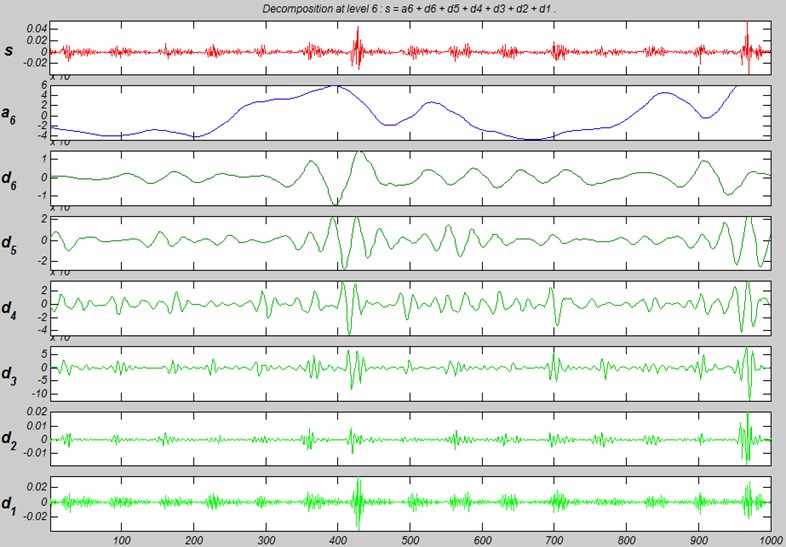
In which $d_i\left(t\right)$ is the details and $a_j\left(t\right)$ is the approximation. Choice of the wavelet function depends on the specific problem being analyzed. In fault diagnosing and monitoring, dabuchies functions ‘dbN’ in which $N$ is the order of the Dabuchy function has been used in many researches. In this paper db4 is chosen as the wavelet function for signal decomposition, and level 6 is chosen.

Standard deviation of details and approximation are used as the characteristic vector for training neural network. Wavelet decomposition of vibration signal from bearing with inner defect is shown in Fig. 5.

Fig. 5Wavelet decomposition of vibration signal from bearing with inner race defect

4. Data normalization

If the acquired data were used directly as the learning pattern inputs to NN, there was the possibility that inputs with higher values, lessens the influence of the inputs with lower values. Also if the raw data was used directly, there was the possibility that neurons saturates. If saturation happens for neurons, the variations in inputs have little or no effect on outputs. This has a negative effect on training. Due to these negative effects, input data are normalized prior to be applied as inputs to the network. Data are normalized between 0 to 1. Input data are normalized according to the following Equation [13]:

where $X_n$ is the normalized data. $x_{min}$ and $x_{max}$ are the maximum and minimum of the data respectively.

5. Processing of vibration signals by NN

5.2. Designing the network

In this research a two layer network which is shown schematically in Fig. 6 has been used.

Fig. 6Schematic of MLPNN

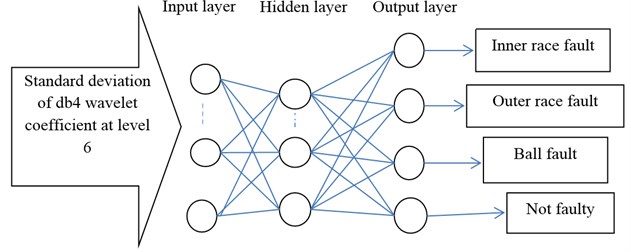
The learning algorithm is back propagation method. Six neurons have been used as input layer. The inputs to these neurons are standard deviation of wavelet coefficients of ($a_6+d_6$), $d_5$, $d_4$, $d_3$, $d_2$ and $d_1$ at 6th level of decomposition with db4. Tan Sigmoid function is considered for the first layer. Four neurons have been used for output layer. Output layer determines the type of bearing under test (fault in inner or outer race, fault in balls and healthy bearing). The target matrix is defined by binary zero and one in which one represents the presence of fault and zero represents lack of fault. For each condition 24 samples were used which makes the total of 96 samples. Vibration signals were divided into three divisions. Two of these divisions were used for training and one division was used for test of the network. The aforementioned network was designed using Matlab software. In the m-file written for this purpose, learning rates, number of epochs and desired error were considered, 0.05, 5000 and 0.00001 respectively. Also the learning function used in this network was considered as batch gradient descent. The flowchart for bearing fault classification is shown in Fig. 7.

In order to choose the best number of neurons in hidden layers, a simulation with different number of hidden layers was done. The results of this simulation with different number of hidden layers are summarized in Table 3.

Fig. 7Bearing fault classification flowchart

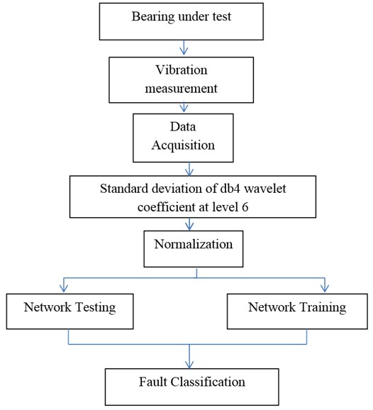
Table 3Performance of different MLPNN structure

Neural network structure number	Number of neurons in hidden layer	Performance percentage
1	5	97.2
2	10	98.26
3	15	98.3
4	20	99.23
5	25	98.73

The best number of neurons in hidden layer are twenty. Fig. 8 shows learning diagram of this network. The convergence pattern as well as the values of mean square error and number of epochs is shown in this figure.

Fig. 8Learning diagram of the MLPNN

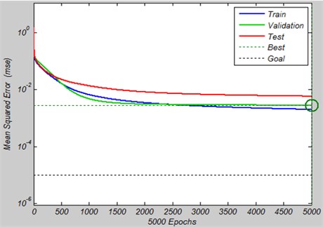
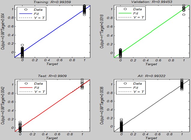
Fig. 9 shows the correlation coefficient of output of network and target data. In Fig. 9 output of the network are shown as circles. The best linear fit is represented by dotted line. Total fit is shown by the solid line. The difference between these two lines is very negligible which shows good results.

Fig. 9Correlation coefficient of MLPNN

6. Results discussion

It has been shown that MLPNN is capable of classification of different bearing faults with over 99 % of accuracy by using the feature vector described in section 5.2. The question which may arise for the reader is, this high accuracy result is obtained under controlled environment of laboratory. What will happen to the accuracy of the proposed method if it is going to perform in real life industrial environment? It should be emphasized that this research showed with proper feature selection it is possible to classify different bearing fault with good accuracy. Of course real life environment is much more sophisticated. The possible fault conditions are much more diverse. Different faults maybe present with different severity. Also different faults may occur simultaneously. Therefore if severity of each of the faults for inner race, outer race and balls were considered as low, medium and high, there would be $\text{3}\times \text{3}=\text{27}$ different cases. So the price of considering more realistic situation is consideration of more cases. But as it was possible to classify the simple case of one fault at a time condition, it is also possible to classify the faults in more realistic situations.

7. Conclusion

The most important contribution of this research is using artificial intelligence in fault detection of rotating machineries. NN has been used for fault detection of rolling bearings by using vibration signals. Vibration signals are preprocessed before being applied to the network by discrete wavelet transform. Standard deviation of discrete wavelet coefficient has been used as inputs. Data with the aid of MLPNN with one hidden layer, with four neurons in output layer has been simulated with different number of neurons in hidden layer.

The simulation results showed the 6:20:4 is the proper structure of NN with efficiency over 99 %.