Abstract
In this paper, an inverse method which formed by two parts: Kalman filter and recursive least-square algorithm is applied to solve an identification problem of the inertia force between a cantilever beam and a moving mass. Based on the basic Euler-Bernoulli beam model, the discretized state space model of the cantilever beam and moving mass system, which transform from the differential equations about the inertia force and modal responses of the cantilever beam, is established. Both the recursive inverse method and the traditional least square method are adapted to the none-noise and noise simulation deflection data which are obtained by the finite element method. The results show that although both two algorithms can bring good results in dealing with the none-noise data, the inverse method has stronger ability to estimate the inertia force in the strong-noise environment, where the traditional least square method fails. Finally, a field experiment is conducted and the identification results show that the recursive inverse method can be adapted to estimate the inertia force between the cantilever and moving mass successfully.
1. Introduction
The identification problem of the inertia force between the cantilever beam and moving mass is very important to many scientific and engineering fields such as structure engineering. By obtaining the accurate identification result, some important parameters of cantilever beam structure can be accessed to. However, if sensors are put between cantilever beam and moving mass, it will damage the structure condition and the inertia force detected in this way won’t be accurate. Therefore, a lot of indirect methods are applied to this identification problem.
A lot of methods to inertia force or moving loads identification problems have been established by the former researchers and some of these methods are based on the classic Euler-Bernoulli beam model. T. H. T. Chan applies the Interpretive Method I (IMI) [1] and Interpretive Method II (IMII) [2] to estimate the moving loads on the bridge structure according to the modal response. S. S. Law adapts Frequency-Time Domain Method (FTDM) [3] and Time Domain Method (TDM) [4], which use the inertia force spectrums in frequency domain and modal superposition principle in time domain respectively, to identify the moving force between the moving objects and the simply supported beam structure. Minzhuo Wang [5] modified the IMII and proposed an adaptive method based on wavelet decomposition, making it suitable to be applied to the inertia force identification problem between the cantilever beam and moving mass. However, this adaptive method has bad performance in the strong noise environment, which makes it not practical in the field experiments.
R. E. Kalman [6] proposed Kalman filtering technique in 1960. Kalman filter has a strong ability to estimate the system status in a strong noise-interference environment [7] and therefore, it has been widely used in many scientific and engineering fields. P. C. Tuan [8] proposed recursive inverse method, which consists of two parts: Kalman filter part and recursive least squares method part, to solve the input heat inverse estimation problems, which will coast much more resources, such as computing time and memory if finite element method is applied. The identification results are accurate and stable under the interference of the noise. C. K. Ma [9] adapted this recursive inverse method to solve some identification problems in many different mechanical structures, such as the estimation of the input force of beam structure or cantilever plate. However, the input forces estimated in these problems are position static and therefore the mathematical model in these problems are not suitable in the identification problem of the inertia force between cantilever beam and moving mass.
In this paper, the basic model proposed by Minzhuo Wang is modified, the discretized state space model of the cantilever beam and moving mass system is proposed and the recursive inverse method is applied to estimate the inertia force between them. The validity of combination of this identification model and method will be tested by the none-noise and noise simulation numerical data and the data obtained by the field experiments.
2. Mathematical model of the problem
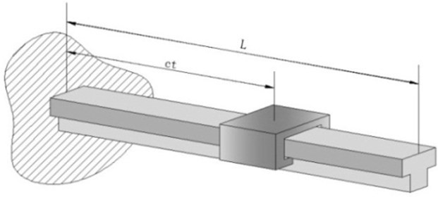
The interaction process between beam structure and moving mass or moving loads is very complex and Euler-Bernoulli beam model can provide an accurate and efficient description of it because the computational complexity of this model is not high. Therefore, the Euler-Bernoulli beam model is chosen in this paper to be the basic model to build up the connection between the inertia force and modal displacements of the cantilever structure. The model of cantilever beam, whose length is , is shown in Fig. 1 and a mass is moving on it at constant speed .
Fig. 1Model of Cantilever
2.1. Differential equations of modal responses and inertia force of cantilever
The differential equation of the deflection of an Euler-Bernoulli beam is given as below [1]:
where is a constant of mass per unit length of cantilever, is the beam deflection at point and time , is a constant of flexural stiffness of cantilever, is the Dirac delta function, is the time-varying inertia force. Because the interaction surface between the cantilever and moving mass is very smooth and is lubricated by lubricating oil, the damping of the motion process can be neglected.
Based on the modal superposition principle, the solution of Eq. (1) can be written as:
where are the modal displacements of the beam structure.
Substitute Eq. (2) to Eq. (1) and each side of Eq. (1) is multiply by , which is the mode shape function. Then integrate the equation with respect to between 0 and , use the properties of Dirac delta function and the boundary conditions of simple supported beam:
the resultant equation can be obtained as:
where:
are the modal frequency of the simple support beam at the -th modal.
However, the boundary conditions of cantilever beam are different from simple support beam and Eq. (3) should be modified as [5]:
What’s more, the modal frequency and vibration modal function of the cantilever beam can only be accessed as approximate value by numerical calculation methods because it can’t be obtained as any analytical form. The frequency equation of cantilever beam is given as [10]:
and the modal function of cantilever beam can be obtained as below:
where is the distance from the sampling points to the start point.
By combining Eq. (4) and Eq. (6), the differential equation of the modal response and time-varying inertia force can be obtained as:
where is the -th modal displacement and is the -th accelerate of the modal vibration of the cantilever, is the maximum order of modal, is the distance between the sampling point and the start point of the cantilever at -th sampling moment.
2.2. Discretized state function of the identification system
Eq. (7) can be rewriten as follow:
where and are the vector of the acceleration and displacement of modal vibration respectively, is the matrix of the modal frequency, is the matrix of modal function and is the inertia force between cantilever beam and moving mass.
The differential equation Eq. (8) can be transform to the continuous-time state equations as below:
and the measurement equation can also be given as:
where , , , is the measurement matrix and is the observation vector.
Eq. (9) can be discretized over time intervals of length with process noise input as follow:
where is the state vector of the system, is the state transition matrix, is the input matrix, is the inertia force between cantilever and moving mass which is going to be estimate and is the input system noise which is assumed to be zero mean and white with variance , where is the process noise covariance and is the Dirac delta function.
The measurement noise also should be considered and therefore Eq. (10) can be discretized as follow:
where the observation vector is:
and the measurement noise vector:
is assumed to be zero mean and white. The variance of is:
where the elements is the standard deviation of measurement noise of .
2.3. Recursive algorithm of inertia force identification
The recursive identification algorithm consists of two parts: Kalman filter part, which is adapted to calculate the residual innovation sequence, and recursive least-square estimation part, which estimates the inertia force between cantilever and moving mass.
The Kalman filter part is given as:
The recursive least-square estimation part is given as:
where is the state prediction without considering the system input , is the state updated estimation, is the covariance of state prediction, is the updated state covariance, , , and are the Kalman gain, covariance and innovation, respectively, is the gain of recursive least-square algorithm, is the error covariance of the estimation of inertia force, and are the sensitivity matrices. What’s more, there is a scalar parameter , which is between 0 and 1, can adjust the performance of the algorithm [8]. When 1, the algorithm becomes to be the regular sequential least-square algorithm. For , it can affect the ability of noise elimination and fast adaption to the signal of the algorithm. If is close to 1, it has a very strong ability to estimate the inertia force from the data affected by the noise, however it will lose its fast adaptive capability. If is close to 0, it can track the fast-varying signal but the identification results will strongly affected by the noise. Therefore, we need a compromising between the fast adaptive capability and the noise elimination capability. The value of should be decided carefully based on the noise the signals have and adaptive capability we need.
The detailed derivation of this estimation algorithm can be found in Tuan’s work [8].
The identification procedure of inertia force between cantilever and moving mass by using the recursive inverse method are illustrated as bellow:
(i) Measure the vibration data of the cantilever, transform it to the modal response and form the observation vector .
(ii) Obtain the innovation covariance , Kalman gain , innovation by using the Kalman filter.
(iii) Calculate the inertia force by substituting , , and into the recursive least-square algorithm.
3. Numerical simulation results
The viability of the recursive inverse method is tested by comparing the identification results to the numerical results calculated by the finite element method (FEM). The parameters of our cantilever model are: the length is 1.5 m, the constant flexural stiffness is 3.42∙105 Nm2 and the constant mass per unit length is 7.8∙103 kg/m3. The sampling frequency is 10 KHz.
For evaluating the effectiveness of the algorithm, a criterion called relative percentage error (RPE) [2], which can express the accuracy of the algorithm across the entire identification progress by comparing the identification results with the numerical results, is introduced as follow:
The initial parameters of the recursive inverse method are set as zeros:
Because and are usually unknown before the identification process start, they can be set as very large value as follow [8]:
and therefore, some initial identification results should be “ignore”, which won’t make a big loss because the algorithm converge very fast and the value of and will soon converge to the reasonable value.
The process noise covariance is set as 10-4, and based on the experiment experience, the measurement noise is set as:
As it mentioned above, the value of scale parameter is very important to the performance of the algorithm. Because the vibration data of the cantilever beam doesn’t vary fast and the data will be affected by the measurement noise, the scale parameter is set as 0.4.
3.1. None-noise data simulation
As it shown in the previous study [11], the recursive inverse method can estimate the inertia force between the cantilever and moving mass very accurately in the none-noise simulation environment. The effectiveness of the recursive inverse method has been tested in three situations with different velocities of moving mass: 5 m/s, 10 m/s and 20 m/s. The RPE value of three tests is shown in Table 1 and the identification results are shown in Fig. 2 4.
As it shown in the Table 1, even though there is a very short delay and some jitters at the beginning of the identification process, the algorithm can estimate the inertia force based on the none-noise deflection data very accurately.
Table 1The RPE of the identification results (none-noise simulation)
Velocity of moving mass (m/s) | RPE |
5 | 0.68 |
10 | 2.05 |
20 | 6.23 |
Fig. 2The identification result (c= 5 m/s)
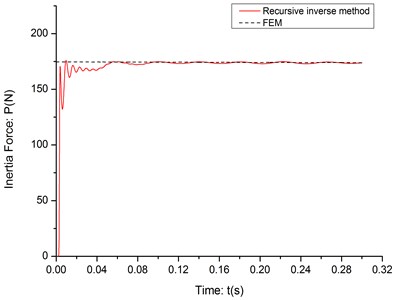
Fig. 3The identification result (c= 10 m/s)
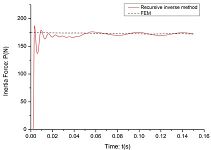
Fig. 4The identification result (c= 20 m/s)
3.2. Noise data simulation
As it mentioned above, the recursive inverse method has a good performance in dealing with the none-noise deflection data of the cantilever beam. However, the deflection data obtained from the field experiment will be affected by the measurement noise and therefore, the capability of reducing the effect of noise is very important for the algorithm.
In order to test the recursive inverse method’s capability of dealing with the noise data, Gaussian noise is added to the none-noise simulation deflection data to imitate the data obtained from the sensors in field experiments. Modified IMII method proposed by Minzhuo Wang [5] is also introduced here to provide contrast.
The recursive inverse method is adapted in two different situations with different measurement noise intensity: the standard deviations of measurement noise are 10-7 and 10-6, which match the measurement noise of two kinds of sensors in our laboratory.
The identification results are shown in Fig. 5-6 and RPE are listed in Table 2.
As it shown in the Fig. 5-6, the recursive inverse method has a very strong ability to identify the inertia force between the cantilever and moving mass in the strong noise environment, where the IMII method fails. At the initial part of the identification process, the results is very unstable because the deflection is very small when the mass has just moved onto the cantilever and the noise data will “submerge” the true deflection data. What’s more, the algorithm itself has not converged yet and some parameters are not stable, either. As the mass moves forward, the deflection of cantilever becomes more severe and the algorithm soon converge, which make the recursive inverse method can estimate the inertia force very accuracy.
Fig. 5The identification result (c= 10 m/s, σ= 10-7)
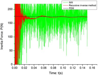
Fig. 6The identification result (c= 10 m/s, σ= 10-6)
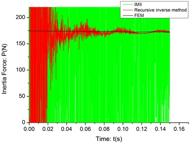
Table 2The RPE of the identification results (noise simulation)
Standard deviation of noise | RPE | |
Recursive inverse method | Modified IMII method | |
10-7 | 2.3375 | 20.6371 |
10-6 | 11.7648 | 215.3404 |
4. Field experiment
In order to verify the feasibility of the recursive inverse method besides the simulation results, a field experiment is designed and conducted.
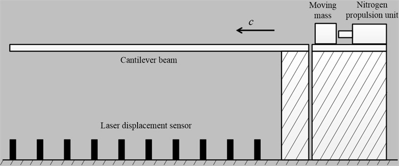
4.1. Experiment setup
As it shown in Fig. 7, a set of experimental apparatus consists of cantilever and moving mass, whose parameters are the same as mentioned in section 3, are build up. A nitrogen propulsion unit is designed to provide the initial impact to the moving mass. Ten laser displacement sensors (Keyence, LK-G400) are evenly placed under the cantilever beam that the length between each of two sensors is 150 mm. The measurement noise of the laser displacement sensor is tested before the experiment and the standard deviation of its measurement noise is approximately equal to 10-7. Data acquisition instrument (Dewetron 1201) is used to provide the sync signals to the laser displacement sensors and record the deflection data of cantilever.
The contact surfaces between the cantilever beam and moving mass are manufactured very smooth and the lubricating oil is added between the surfaces, therefore, the moving damp can be neglected and the velocity of the moving mass can be assumed to be constant. In fact, in the prep experiments, a high speed camera (IDT-Y3) is set up to record the motion process of the mass and a motion analysis software (ProAnalyst) is used to calculate the speed of the moving mass. The results show that the decrease amount of the speed is very small and therefore the model assumption that the damp can be neglected is appropriate.
As soon as the mass moves on the cantilever, the laser displacement sensors begin to record the displacement of the cantilever and a high speed camera (not be shown in Fig. 8), which is synchronous with the data acquisition device, is set at the fixed end of the cantilever to record the exact moment the mass move out the fixed end of the cantilever beam which can be seen as the start signal of the data recording.
Fig. 7The experiment schematic diagram
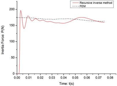
4.2. Experiment results
Three experiments with different mass velocity, 10 m/s, 15 m/s and 20 m/s, are conducted and the identification result of the inertia force of each experiment is shown in Fig. 8-10.
Fig. 8The experiment identification result (c= 10 m/s)
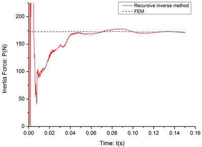
Fig. 9The experiment identification result (c= 15 m/s)
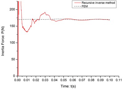
Fig. 10The experiment identification result (c= 20 m/s)
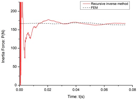
Table 3The RPE of the experiment identification results
Velocity of moving mass (m/s) | RPE |
10 | 1.145 |
15 | 1.247 |
20 | 1.739 |
As it can be seen in the Fig. 8-10, the initial part of the identification process is very unstable, even much more unstable than the noise-data simulation results and it is obvious not caused by the signal noise or instability of the algorithm. After checking the deflection data, it is found that when mass has just moved on the cantilever, it will bring an impact to the structure and even when it pass the fixed end, the impact wave can’t vanish in such short time and it will interfere the deflection of cantilever beam. After the impact wave vanish in a short period, the recursive inverse method can identify the inertia force between cantilever and moving mass very accurately. The RPE of the stable part of each identification result is listed in Table 3.
5. Discussion
In the field experiments, the initial part of the identification process is very unstable because when the mass has just moved on the fixed part of cantilever, the impact wave can’t be vanished before it moves out the fixed end of the cantilever. If the fixed part can be extended, moving mass will be able to stay in the fixed part of the cantilever for a longer time and the impact wave can be vanished which will be helpful to the identification.
The whole identification model is based on the assumption that the velocity of the moving mass is stable and as mentioned in section 4.1, it has been proved by the prep experiment result that our experiment apparatus meet this assumption. However, if the length of the cantilever beam is much longer or contact surface are not smooth, this assumption can’t be correct because the mass will lose some energy in the process of moving and the identification model should be modified in that case.
As it mentioned above, a compromise between the fast adaptive capability and strong noise elimination capability of the recursive inverse method is needed when choose the value of scale parameter . In the case of this paper, the noise elimination capability is considered to be more important than the fast adaptive capability because the inertia force doesn’t change dramatically and signals from the sensors could have a lot of noise. If the identification parameter changes a lot during the process, the noise elimination capability should be weakened by adjusting the scale parameter in order to improve the fast adaptive capability.
In order to obtain the deflection data of the cantilever beam, the sensors should be chosen very carefully. The sensors should have a high resolution because the deflection of the cantilever beam is very small. What’s more, the sensors should be very stable and the measurement noise of the signal can’t be very severe.
6. Conclusions
In this paper, the recursive inverse method is adapted to identify the inertia force between the cantilever beam and moving mass. A new identification model is formed and an experiment is set up to obtained the deflection data of the cantilever. The feasibility of the identification model and method is verified by the numerical simulation results (none-noise data and noise data) and the field experiment results.
Future work will focus on the improving of the experiment setup and the identification method itself.
References
-
T. H. T. Chan, L. Yu, S. S. Law, T. H. Yung. Moving force identification studies, I: theory. Journal of Sound and Vibration, Vol. 247, Issue 1, 2001, p. 59-76.
-
T. H. T. Chan, S. S. Law, T. H. Yung, X. R. Yuan. An interpretive method for moving force identification. Journal of Sound and Vibration, Vol. 219, Issue 3, 1999, p. 503-524.
-
S. S. Law, T. H. T. Chan, Q. H. Zeng. Moving force identification: a frequency and time domains analysis. Journal of dynamic systems, Vol. 121, Issue 3, 1999, p. 394-401.
-
S. S. Law, T. H. T. Chan,Q. H. Zeng. Moving force identification: a time domain method, Journal of Sound and Vibration, Vol. 210, Issue 1, 1997, p. 1-22.
-
Qiang Chen, Minzhuo Wang, Hao Yan, Haonan Ye, Guolai Yang. An adaptive method for inertia force identification in cantilever under moving mass. Journal of Vibroengineering, Vol. 14, Issue 3, 2012, p. 1052-1058.
-
R. E. Kalman. A new approach to linear filtering and prediction problems. Journal of basic Engineering, Vol. 82, Issue 1, 1960, p. 35-45.
-
R. G. Brown, P. Y. C. Hwang. Introduction to random signals and applied Kalman filtering. John Wiley & Sons, New York, 1992.
-
P. C. Tuan, C. C. Ji, L. W. Fong, W. T. Huang. An input estimation approach to on-line two-dimensional inverse heat conduction problems. Numerical Heat Transfer, Vol. 29, Issue 3, 1996, p. 345-363.
-
C. K. Ma, J. M. Huang, D. C. Lin. Input forces estimation of beam structures by an inverse method. Journal of Sound and Vibration, Vol. 259, Issue 2, 2003, p. 387-407.
-
Jingbo Liu, Xiuli Du. Structural Dynamics. China Machine Press, Beijing, 2005.
-
Qiang Chen, Hao Yan, Minzhuo Wang, Haonan Ye. Inertia Force Identification of Cantilever under Moving-Mass by Inverse Method. TELKOMNIKA Indonesian Journal of Electrical Engineering, Vol. 10, Issue 8, 2012, p. 2108-2116.
About this article

This work was supported in part by the Major State Basic Research Development Program of Republic of China (No. 613116).
