Abstract
The stability of high-speed spindle system affects the surface finish and tool life directly, which is an important factor to evaluate its performance. Meanwhile, the spindle dynamics and cutting stability are affected by the structure and dynamics of spindle-holder-tool joints significantly. The joints are simplified as the distribution-spring, and the FEM modeling process of spindle system is proposed based on the thought of parallel rotor system. Taking a vertical machining center as example, the effectiveness of the modeling method is verified. Starting from the stability evaluation criteria and different ways of getting FRF, the influence factors of unconditional and conditional stability regions are analyzed. Based on the proposed model, the influence laws of cutting stability on cutting force amplitude and speed are characterized by the three-dimensional lobes, limit cutting depths and lobe intersections, which provide the theoretical basis for optimizing the processing and improving the cutting stability.
1. Introduction
The connections between spindle, holder and tool are the power and precision transmission called spindle-holder-tool joints. The spindle-holder joint is Conic Surface and the holder-tool joint is cylindrical surface, the characteristic of which are high geometric accuracy, high repeated loading and high stiffness for spindle processing safely and reliably [1]. The spindle-holder-tool joints affect the spindle dynamic characteristic significantly. Erturk [2] discovered the spindle-holder-tool joints affected the modal of spindle making the inherence frequencies and modal vibration changed. Xing [3] and Zhengjia [4] researched the modeling method of spindle and joints. Therefore, the spindle system modeling method considering spindle-holder-tool joints characteristics should be researched for predicting the spindle dynamic effectively.
However, the researchers pay high attention to rolling bearing modeling but neglect the influence of spindle-holder-tool joints on spindle dynamic characteristics during the study at present. Rantatalo [6], Altintas [7] and Tu [8] explored influence of spindle dynamic characteristic on gyroscopic moment, shaft and bearing centrifugal force inducing by high speed. The angular contact ball bearing model was emphasized, but other joints were neglected. Shin [9] and Altintas [10] built the spindle-holder-tool joints model rigid connection. Rturk [11] considered the spindle-holder-tool joints concentrated spring model as bearing simplified model.
Machine tools or machining centers have the ability of resisting vibration during cutting process (including the forced vibration and self-excited vibration) called cutting stability, or the vibration resistance. The chatter of machine tools derives from self-excited mechanism during the manufacturing process, which affects the removal rate, process accuracy, production efficiency and tool service life greatly. The stability receives more and more attentions because of high-speed machining widely used in automotive, mold, aerospace and other precision manufacturing.
Insperger [1] created the stability of single DOF milling system by semi-discretization method. Tlusty [13] built the stability lobe diagrams during milling process by time-domain simulation. Schmitz [14] and Ahmadi [15] predicted dynamic characteristics and cutting stability of high-speed machining center by substructure. Weixiao [16] proposed limit criterion and analysis method of multiple DOF system on high inherence frequencies under high speed cutting condition.
The researchers explore the affected factors of stability including tool length, tool types and rotation speed with the study deepening. Tlusty [17] discussed the common modal of spindle with long end milling tool and analyzed the influence of stability on different tool lengths with changing speeds. Smith [18] and Davies [19] studied the stability of high slenderness ratio, low radial cutting depth and workpiece mass respectively. Ismail [20], Shin [21] and Altintas [22] predicted stability of non-equal interval cutter, ball end milling cutter and face milling cutter. Schmitz [23] proposed the FRF test method of non-rotation and rotation tool. Qinghua [24] researched the influence of stability on structure parameters.
The accurate dynamic characteristics of spindle system are used to structure designing and stability predicting, which is unable to satisfy the design demand without consideration of spindle-holder-tool joints dynamic characteristics. Therefore, the spindle-holder-tool joints method was built with distributing spring model, and the process of spindle system model is proposed based on the joints model thought of parallel rotor system by FEM. The effectiveness of the model on spindle system dynamics simulating is verified by experiment on a vertical machining center. From the stability evaluation criteria, the conditional stability region is also a key to process stability. Based on the proposed model, the influence laws of cutting stability on cutting force amplitude, speed and damping ratio are characterized by the three dimensional lobes, limit cutting depths and lobe intersections, which provide the theoretical basis for optimizing the processing and improving the cutting stability.
2. Modeling method of spindle-holder-tool joints
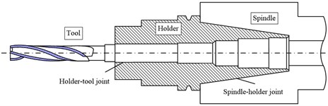
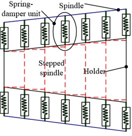
The local enlarge section of spindle-holder-tool is shown in Fig. 1. The joints consist of two parts: the spindle-holder joint is conical surface producing friction force by drawer, which is the part of holder inserting spindle, the holder-tool joint is cylindrical surface positioning by screws, which is the part of tool inserting holder.
Fig. 1Local sectional drawing of spindle-holder-tool joints
2.1. FEM modeling principle of parallel rotors
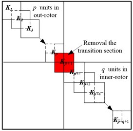
The parallel rotors system consists of inner rotor and outer rotor. The unit nodes are numbered continuous when the rotor system is discrete. A transition section is added at the end of outer rotor, the information of which is given randomly. The assembly process includes giving the mass and stiffness matrixes of all the units firstly, assembling all the matrixes and removing the matrixes of transition section, finally, the mass matrix and stiffness matrix of parallel rotors could be got.
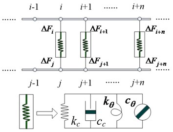
Assuming units in outer rotor and units in inner rotor, there are units in the parallel rotor system and nodes, . The mass and stiffness matrices of each unit are 12×12 orders, which is consist of two nodes and each node owns six degree freedoms. The assembly of adjacent units is shown as Fig. 2. The mass and stiffness matrices of whole system are 6×6 orders, from which the transition section matrices will be removed. The final complete mass and stiffness matrices of parallel rotor are shown as Fig. 3.
Fig. 2Schemes of adjacent unit assembly
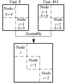
Fig. 3Schemes of parallel rotors assembly
2.2. Dynamic simulation of spindle-holder-tool joints
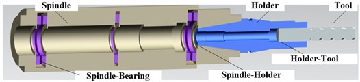
The spindle-holder-tool joints consist of double parallel rotor systems, one is spindle and holder, the other is holder and tool. The sectional drawing of complete spindle system is shown as Fig. 4. Dynamic simulation of joints is illustrated taken the spindle-holder joint as example. The distribution-spring model of spindle-holder joint is shown as Fig. 5 (Fig. 5(a) is the toper joint structure and Fig. 5(b) is the joint FEM).
Fig. 4Sectional drawing of spindle system
Assuming the spindle and holder joint is divided into stepped shafts, in the joint there are nodes, , ,…, on the spindle and , ,…, on the holder, respectively. The coupling forces on the spindle and holder are:
where, and are coupling stiffness and damping matrices at spindle-holder joint, and are the displacement vectors of spindle and holder at the joint, and are the coupling forces at spindle-holder joint, and are node numbers at spindle-holder joint.
The stiffness and damping matrices of spindle-holder joint expressed with and are:
Fig. 5The distribution-spring model of spindle-holder joint
a) Structure
b) FEM
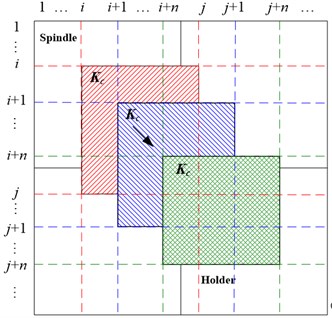
The stiffness characteristic of distribution-spring is shown in Eq. (2) and the damping characteristic is shown in Eq. (3). The assembly method of stiffness on joint is shown in Fig. 6.
Fig. 6Stiffness assembly theory of spindle-holder joint
2.3. Modeling process of spindle-holder-tool joints
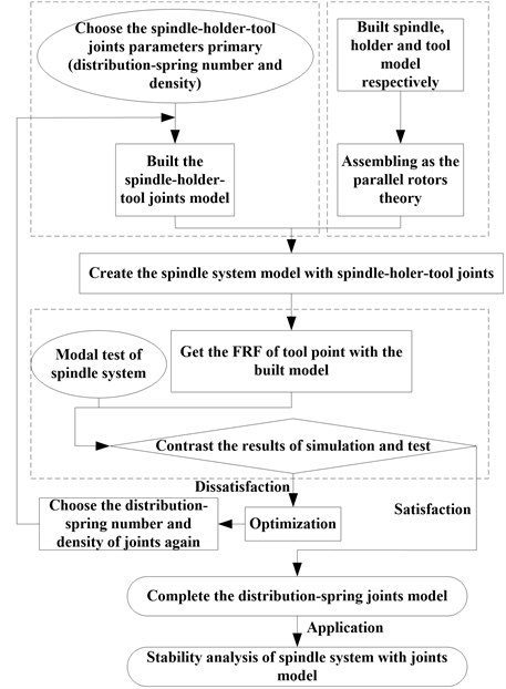
The spindle-holder-tool joints modeling should be combined with the system modeling, which is not independent exit. Based on the parallel rotors idea, the joints are built with distributed spring model. The parameters of spring numbers, density, stiffness and damping are set, the spring numbers and density of which could be amendment with experiment. The modeling process of spindle-holder-tool joints is shown as Fig. 7.
Step 1: building the FEM model of spindle, holder and tool respectively. Firstly, the different sections are divided according to inner and outer diameters, secondly, two transition sections are added at the end of spindle and holder respectively, finally, the nodes of units are numbered continuously including the transition sections.
Step 2: creating the spindle-holder-tool joints model. The spring density, number, stiffness and damping are chosen primary. Then the distribution-spring model is created with the divided units of joints using the spring stiffness and damping. The complete spindle system model will be got assembling the joints and spindle, holder, tool model.
Step 3: the modal test and dynamic simulation. The FRF at tool point of the built model is got though modal analysis, which is verified by modal test. The number and density of distribution-spring will be corrected through the test and simulation results.
Step 4: the model application. The dynamic and stability prediction will be done with the complete spindle model considering the spindle-holder-tool joints.
Fig. 7Modeling process of spindle-holder-tool joints
2.4. FEM of complete spindle system
The high-speed spindle system is established with isoparametric beam element, each unit of which exits 12-DOF including 3 translational DOFs and 3 rotational DOFs on each node. The unit mass, stiffness and damping matrixes are assembled into the dynamic equation of system considering bearing force and spindle-holder-tool joints as follow:
where, is mass matrix; is damping matrix; is stiffness matrix; is damping matrix; is gyroscopic matrix; is coupling stiffness matrix of joints; is stiffness matrix of spindle; is centrifugal stiffness matrix of spindle; is supporting bearing force vector; is hysteretic force vector of spindle-holder-tool; is cutting force vector; is gravity vector; is displacement vector; is displacement vector of node ; , , , , , are 3 translational and 3 rotational DOFs of node .
The FEM model of high-speed spindle system in the free-state is shown as Fig. 8. There are 66 units and 66 nodes in the FEM including 2 transition sections. The structures of spindle system are shown in Table 1 and Table 2. The dynamic parameters of system are: elasticity modulus 2.06×10¹¹ Pa, material density 7850 kg/m3. The FEM of test object is built with 5-distribution-spring connection, 10-distribution-spring connection and rigid connection respectively.
Fig. 8The model of high speed spindle system
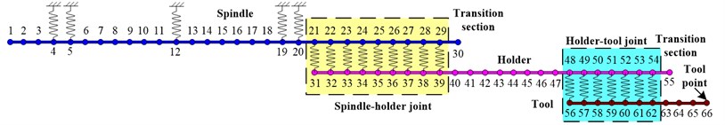
Table 1The size of motorized spindle, mm
No. | No. | No. | |||||||||
1 | 14.50 | 120.00 | 70.00 | 11 | 15.00 | 150.00 | 55.00 | 21 | 11.30 | 129.90 | 43.46 |
2 | 25.00 | 149.90 | 70.00 | 12 | 30.00 | 150.00 | 65.00 | 22 | 11.30 | 129.90 | 46.76 |
3 | 15.00 | 149.90 | 55.00 | 13 | 30.00 | 150.00 | 65.00 | 23 | 11.30 | 129.90 | 50.06 |
4 | 15.00 | 149.90 | 55.00 | 14 | 30.00 | 150.00 | 55.00 | 24 | 11.30 | 129.90 | 53.36 |
5 | 25.00 | 149.90 | 65.00 | 15 | 25.00 | 150.00 | 55.00 | 25 | 11.30 | 129.90 | 56.66 |
6 | 30.00 | 149.90 | 65.00 | 16 | 25.00 | 150.00 | 55.00 | 26 | 11.30 | 129.90 | 59.96 |
7 | 25.00 | 149.90 | 65.00 | 17 | 25.00 | 150.00 | 70.00 | 27 | 11.30 | 88.00 | 63.26 |
8 | 25.00 | 149.90 | 65.00 | 18 | 15.00 | 150.00 | 55.00 | 28 | 11.40 | 88.00 | 66.56 |
9 | 30.00 | 150.00 | 65.00 | 19 | 15.00 | 150.00 | 55.00 | 29 | 5.00 | 88.00 | 69.85 |
10 | 30.00 | 150.00 | 65.00 | 20 | 11.30 | 149.90 | 40.16 |
Table 2The size of holder and tool, mm
Holder | Tool | ||||||||||
No. | No. | No. | |||||||||
1 | 11.30 | 40.16 | 25.00 | 13 | 11.40 | 100.00 | 20.00 | 1 | 10.00 | 32.00 | 0.00 |
2 | 11.30 | 43.46 | 25.00 | 14 | 12.00 | 95.00 | 20.00 | 2 | 10.00 | 32.00 | 0.00 |
3 | 11.30 | 46.76 | 24.00 | 15 | 12.00 | 90.00 | 20.00 | 3 | 10.00 | 32.00 | 0.00 |
4 | 11.30 | 50.06 | 24.00 | 16 | 10.00 | 86.00 | 20.00 | 4 | 10.00 | 32.00 | 0.00 |
5 | 11.30 | 53.36 | 24.00 | 17 | 22.00 | 86.00 | 32.00 | 5 | 10.00 | 32.00 | 0.00 |
6 | 11.30 | 56.66 | 24.00 | 18 | 10.00 | 86.00 | 32.00 | 6 | 10.00 | 32.00 | 0.00 |
7 | 11.30 | 59.96 | 20.00 | 19 | 10.00 | 86.00 | 32.00 | 7 | 11.00 | 32.00 | 0.00 |
8 | 11.30 | 63.26 | 20.00 | 20 | 10.00 | 86.00 | 32.00 | 8 | 8.00 | 30.00 | 0.00 |
9 | 11.40 | 66.56 | 20.00 | 21 | 10.00 | 86.00 | 32.00 | 9 | 18.00 | 25.60 | 0.00 |
10 | 5.00 | 69.85 | 20.00 | 22 | 10.00 | 80.00 | 32.00 | 10 | 18.00 | 25.60 | 0.00 |
11 | 19.00 | 100.00 | 20.00 | 23 | 10.00 | 80.00 | 32.00 | 11 | 20.00 | 25.60 | 0.00 |
12 | 7.40 | 85.00 | 20.00 | 24 | 11.00 | 80.00 | 32.00 | ||||
3. Model verification
3.1. Test object
The modal experiment is done on VMC0540d by hammering to prove the effective of modeling method for spindle-holder-tool joints and the whole spindle system. The results obtained from the experiment, 5-distribution-spring model. 10-distribution-spring model and rigid model will be compared by the frequency response function of tool point.
The test system is set up and shown in Fig. 9. The test object is a spindle system which consists of HCS150 motorized spindle from GMN, BBT50-MEGA32D-165 holder and HLXX32 end milling cutter. The main test equipments include the data acquisition, hammer and vibration sensors in Table 3.
Fig. 9The test system
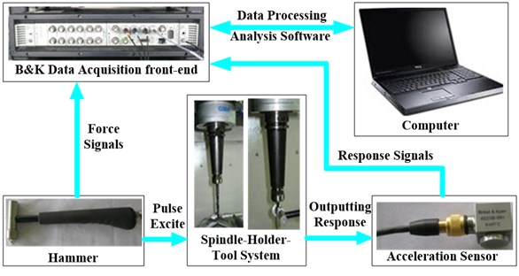
Table 3The instruments used in this test
No. | Name |
1 | B&K 3560-C data acquisition front-end |
2 | PCB 8206-001 54627 modal hammer |
3 | B&K 4525B-001 54072 acceleration sensor |
4 | High-performance notebook computers |
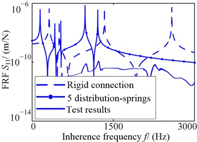
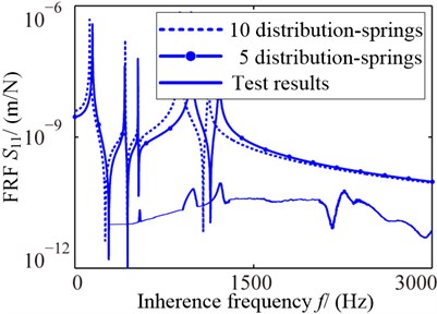
The FRFs at tool point of rigid connection joints, 5-distribution-spring joints and test results are show as Fig. 10(a), and the FRFs of 5-distribution-spring joints, 10-distribution-spring joints and test results are show as Fig. 10(b).
Fig. 10Comparison of different joints models and test results
a) Different model types
b) Different spring density
The inherence frequencies of joints different forms are shown in Table 4 including rigid connection, concentrated spring model, different distribution-spring models and test results. There is no rigid modal in test results. From the Table, the simulation errors of rigid model are largest than other connections from the test results, which is from 82.65 % to 158 %.
The Fig. 10 shows that the FRF of 5-distribution-spring joint model is closer to the test result than 10-distribution-spring model, and also closer than the rigid one. The Table 4 shows that the distribution-spring model results are much closer to the test than the concentrated. For the spring layout form, the 5-distribution-spring joint model are more perfect than the 10-distribution-spring joints for the size of joints which is closer to the other unit in the model, which illustrates the influence of FRF on distribution-spring form is obvious and the 5-distribution-spring joint model is verified effectively.
Table 4Comparison of inherent frequencies of different joints models and test results
Order Model types | Rigid modal | Elastic modal | ||||||
First | Second | First | Second | Third | Fourth | |||
Rigid connection | / Hz | 315.52 | 502.32 | 1 336.4 | 2 579.7 | 2 974.0 | 4 133.4 | |
% | – | – | 143 % | 158 % | 142 % | 82.65 % | ||
Concentrated spring | / Hz | 171.9 | 426.81 | 532.95 | 970.46 | 1 382.4 | 2 187.2 | |
% | – | – | –3.1 % | –2.954 % | 12.57 % | –3.358 % | ||
Distribution springs | 5 units | / Hz | 148.56 | 419.67 | 530.95 | 978.33 | 1 212.3 | 2 277 |
% | – | – | –3.46 % | –2.167 % | –1.278 % | 0.618 4 % | ||
10 units | / Hz | 125.4 | 423.92 | 531.75 | 880.61 | 1 120.8 | 2 327.1 | |
% | – | – | –3.318 % | –11.94 % | –8.73 % | 2.83 % | ||
Test results | / Hz | – | – | 550.6 | 1 000.7 | 1 228.9 | 2 263.4 | |
4. Influence factors and prediction method of cutting stability
4.1. Influence factors of stability
The cutting stability is evaluated through lobe diagram generally, which is characterized by cutting limit depth, as Eq. (5) [14]:
where, is the maximum cutting depth without chatter, is cutter teeth, is cutting force coefficient in feed direction, is real part of FRF, is angular frequency of negative FRF.
From the Eq. (5), the zone under is unconditionally stability zone affected by , and . The system will chatter when the cutting depth is higher than the under specific speed theoretically. However, the emergence of conditionally stability zone will make the system stability with higher cutting depth. The conditionally stability zone is affected by lobe distribution, which still is controlled by FRF. Therefore, the FRF is a significant factor of cutting stability.
The FRF of system could be obtained by direct method and inherent characteristics method except modal test. The direct method is using the concept of frequency response function, which is the Laplace transformation ratio of response (or output) and excitation (or input) when the initial condition is zero in a linear constant system as Eq. (6):
where, is Laplace transformation ration of response, is Laplace transformation ration of excitation, is frequency response function of system.
The inherent characteristics method begins with the essence of FRF. When the system equation is Laplace transformation of two sides is , then there is:
where, is transfer function matrix of system, is Laplace transformation of excitation vector, is Laplace transformation of response vector:
Take the Eq. (8) into Eq. (7), , the displacement FRF of excitation at , and response at is as follow:
where, and are the order modal shape of and , is damping ratio, is inherence angular frequency, is excitation angular frequency.
From the Eq. (7) to (9), there are many influence parameters on FRF including excitation , response , mass , stiffness , damping , modal shape , inherence frequency , damping ratio , even the spindle-holder-tool joints dynamic characteristics discussed in the paper above and rotational speed verified by [15]. This paper focuses on the influence of cutting stability on cutting force (excitation) and speed (process condition) with specific system.
4.2. Stability prediction process
Based on modeling the system with distribution-spring joint model and solving the FRF, the lobe diagram will be drawn as follow:
Step 1: the FRF is divided into two parts: the real and imaginary part as . Solve the value of to satisfy and obtain the according to the and Eq. (5).
Step 2: positive and negative of imaginary part is judged by . If then the phase angle of system will be or . The rotational speed will be got according to , and .
Step 3: the and will be obtained in each lobe. The lobe diagram will be formed through drawing several lobes in the picture.
5. Influence rules of cutting stability
5.1. Influence of cutting force
The cutting force during the process is simulated by harmonic force, and the influence rule of stability is analyzed by changing the force amplitude. The three-dimensional lobe diagram with changing forces is shown as Fig. 11(a) and stability lobe diagram under two different forces is shown as Fig. 11(b), both of which show the limit cutting depth reduces as the force increases and the conditional zone affected by the force.
The limit cutting depths and lobe intersections correspond to the critical speeds changing with forces are shown as Fig. 12. From the Fig. 12(a), the limit cutting depths are reduced as the force increasing, which are affected greatly when the cutting force is small or gently when it is bigger. The first intersection is the one of 0 and 1, then the second intersection is the one of 1 and 2 from the Fig. 12(b), which shows the intersections move to the left as the force increasing. Therefore, the conditional zones are changed with the forces.
Fig. 11Stability lobes of different cutting forces
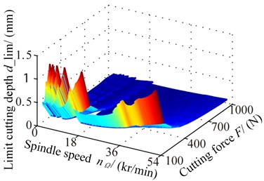
a) Three-dimensional lobe
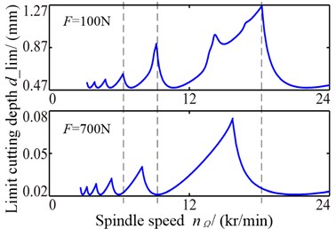
b) Lobe under different cutting forces
Fig. 12Stability influence rules of cutting forces
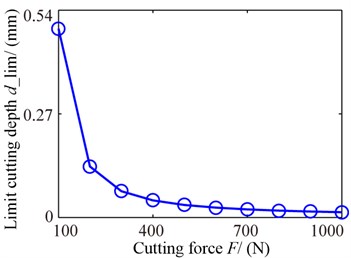
a) Minimum limit cutting depth
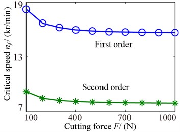
b) Lobe intersection
5.2. Influence of rotational speed
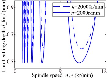
The three-dimensional lobe diagram of stability with changing rotational speeds is shown as Fig. 13(a) and stability lobe diagram under two different sweep speeds are shown as Fig. 13(b). As the rotational speed rise, the limit cutting depths increase, which illustrates the cutting stability strengthen.
Fig. 13Stability lobes of different sweep speeds
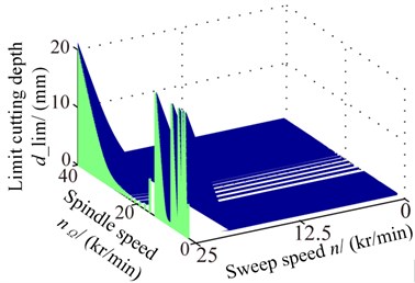
a) Three-dimensional lobe
b) Lobe under different sweep speeds
The limit cutting depths and lobe intersections correspond to the critical speeds changing with rotational speed are shown as Fig. 14. From the Fig. 14(a), the limit cutting depths are enlarged as the speed increasing, but the first order remarkably and the secondly order is slow. Fig. 14(b) shows the intersections move to the right as the speed increasing, which states the conditional zones change complicated.
Fig. 14Stability influence rules of sweep speeds
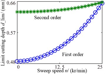
a) Minimum limit cutting depth
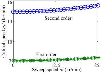
b) Lobe intersection
6. Conclusions
In this paper, the dynamic model of spindle-holder-tool joints has been built and assembled into the complete high-speed spindle system model. From the practical viewpoint of application, the influence rules of cutting force and speed have been investigated. Based on the modeling and application results, the following conclusions can be drawn:
(1) The model of spindle-holder-tool joints were created with distribution-spring method, the joints model was assembled into the whole spindle system model and the modeling process was established.
(2) The distribution-spring method was verified by other simulation method and test, and the arrangement form of distribution-spring method was not the better the denser, but its length was close to other units because of the joints model truly reflect the actual one.
(3) The novel viewpoint was proposed that the conditional zone was as significant as unconditional zone in improving the stability. From the analysis of influence rules, the stability declined as the cutting force rising, the unconditional zone was expanded as the rotational speed increasing but the conditional zone moved to the right, which implies the influence of speed on stability is complicated, so the particular speed needs particular analysis.
From the investigation, the distribution-spring method is the closest arrangement form to the real spindle-holder-tool joints. How to apply the joints model into the nonlinear stability evaluation and influence parameters analysis may be a good research subject in the future.
References
-
AI Xing High speed machining technology. Beijing, National Defence Industry Press, 2003.
-
Erturk A., Ozguven H. N., Budak E. Effect analysis of bearing and interface dynamics on tool point FRF for chatter stability in machine tools by using a new analytical model for spindle-tool assemblies. International Journal of Machine Tools and Manufacture, Vol. 47, 2007, p. 23-32.
-
Zhang Song, Ai Xing, Zhao Jun FEM-based parametric optimum designing of spindle/tool holder interfaces under high rotational speed. Chinese Journal of Mechanical Engineering, Vol. 40, Issue 2, 2004, p. 83-87.
-
Cao Hongrui, He Zhengjia Dynamic modeling and model updating of coupled systems between machine tool and its spindle. Chinese Journal of Mechanical Engineering, Vol. 48, Issue 3, 2012, p. 88-94.
-
Li Songshen, Chen Xiaoyang, Zhang Gang, et al. Analyses of dynamic supporting stiffnesss about spindle bearings at extra high-speed in electric spindles. Chinese Journal of Mechanical Engineering, Vol. 42, Issue 11, 2006, p. 60-65.
-
Rantatalo M., Aidanpaa J. O., Goransson B., Norman P. Milling machine spindle analysis using FEM and non-contact spindle excitation and response measurement. International Journal of Machine Tools and Manufacture, Vol. 47, 2007, p. 1034-1045.
-
Cao Yuzhong, Altintas Y. A general method for the modeling of spindle-bearing systems. Journal of Mechanical Design, Vol. 126, Issue 6 2004, p. 1089-1104.
-
Lin Chiwei, Tu J. F., Kamman J. An integrated thermo-mechanical-dynamic model to characterize motorized machine tool spindles during very high speed rotation. International Journal of Machine Tools and Manufacture, Vol. 43, 2003, p. 1035-1050.
-
Li Hongqi, Shin Y. C. Analysis of bearing configuration effects on high speed spindles using an integrated dynamic thermo-mechanical spindle model. International Journal of Machine Tools and Manufacture, Vol. 44, 2004, p. 347-364.
-
Altintas Y., Cao Yuzhong Virtual design and optimization of machine tool spindles. CIRP Annals, Manufacturing Technology, Vol. 54, 2005, p. 379-382.
-
Erturk A., Ozguven H. N., Budak E. Analytical modeling of spindle–tool dynamics on machine tools using Timoshenko beam model and receptance coupling for the prediction of tool point FRF. International Journal of Machine Tools and Manufacture, Vol. 46, 2006, p. 1901-1912.
-
Insperger T., Mann B. P., Stépán G., et al. Stability of up-milling and down-milling, part 1: alternative analytical methods. International Journal of Machine Tools and Manufacture, Vol. 43, 2003, p. 25-34.
-
Smith S., Tlusty J. Efficient simulation programs for chatter in milling. Annals of the CIRP-Manufacturing Technology, Vol. 42, Issue 1, 1993, p. 463-466.
-
Schmitz T. L. Predicting high-speed machining dynamics by substructure analysis. Annals of the CIRP, Vol. 49, Issue 1, 2000, p. 303-308.
-
Ahmadi K., Ahmadian H. Modeling machine tool dynamics using a distributed parameter tool-holder joint interface. International Journal of Machine Tools and Manufacture, Vol. 47, 2007, p. 1916-1928.
-
Tang Weixiao Research on high-speed machining stability and dynamic optimization. Jinan, Shandong University, 2005.
-
Tlusty J. Dynamics of high-speed milling. Journal of Engineering for Industry, Vol. 108, 1986, p. 59-67.
-
Smith S., Winfough W. R., Pratt J. R., et al. The effect of tool length on stable metal removal rate in high-speed milling. Annals of the CIRP, Vol. 47, Issue 1, 1998, p. 307-310.
-
Davies M. A., Dutterer B., Pratt J. R., et al. On the dynamics of high-speed milling with long, slender endmills. Annals of the CIRP, Vol. 47, Issue 1, 1998, p. 55-60.
-
Ismail F., Soliman E. A new method for the identification of stability lobes in machining. International Journal Machine Tools Manufacture, Vol. 37, Issue 6, 1997, p. 763-774.
-
Jensen S., Shin Y. Stability analysis in face milling operations. Journal of Manufacturing Science and Engineering, Vol. 121, Issue 4, 1999, p. 600-614.
-
Altintas Y., Engin S., Budak E. Analytical stability prediction and design of variable pitch cutters. Transactions of ASME Journal of Manufacturing Science and Engineering, Vol. 121, Issue 2, 1999, p. 173-178.
-
Schmitz T. L., Ziegert J. C., Stanislaus C. A method for predicting chatter stability for systems with speed-dependent spindle dynamics. Aerospace Engineering, Vol. 32, 2004, p. 17-24.
-
Song Qinghua High-speed milling stability and machining accuracy. Jinan, Shandong University, 2009.
-
Altintas Y. Manufacturing automation – metal cutting mechanics, machine tool vibrations and CNC design. Cambridge University, 2002.
-
Wang Bo, Sun Wei, Wen Bangchun The finite element modeling of high-speed spindle system dynamics with spindle-holder-tool joints. Journal of Mechanical Engineering, Vol. 48, Issue 15, 2012, p. 83-89.
-
Sun Wei, Wang Bo, Wen Bangchun Comparative analysis of dynamics characteristics for static and operation state of high-speed spindle system. Journal of Mechanical Engineering, Vol. 48, Issue 11, 2012, p. 146-152.
About this article

This work supported by the National Natural Science Foundation of China (50905029), National Science Foundation for Postdoctoral Scientists of China (2013M541239), Research Foundation of Education Bureau of Liaoning Province, China (L2013115), Fundamental Research Funds for the Central Universities of China (N110603004).
