Abstract
The study of vibrations induced by a passing train is of utmost importance to understand better this phenomenon and to design efficient mitigation measures. Within all the techniques used to model vibrations, finite element methods allow introducing in the model detailed characteristics of the real vehicle-train-soil system. However, the accuracy of the results is linked to how detailed the real elements implemented in the model are and consequently, with the computing time. In this paper a three-dimensional finite element method to predict vibrations is developed and validated with real field-measured data. Then, different scenarios are represented to assess the efficiency of the model linking the quality of the results obtained with the calculation time required in each case. Finally, a reflection regarding the constitutive model of the materials when working with finite element models is done.
1. Introduction
Railway has demonstrated to be an efficient transport mean both for freight and people transport. The high capacity and the low impact on the environment and pollution when it is compared to other transport means have encouraged the development of new railway networks in recent decades and the adaptation of the existing ones to the current needs as well.
Nevertheless, within the main drawbacks of railway transport the externalities are found. Externalities include vibrations that, generated in the wheel-rail contact propagate through the railway surroundings and may cause damage on the buildings or nuisance to people who live or work close to the track. One of the first experimental studies about the vibration effects on buildings was performed by Dawn and Stanworth [1] and propagation speed of the vibration wave through the ground was identified as a key parameter in the propagation. Experimental research was extended by Degrande and Schillemans [2] to high speed lines measuring accelerations in the track and in the surrounding soil. Field researches such as seen before promoted the development of mathematical models to explain the phenomenon and therefore predict vibrations and propose mitigation measures. These mathematical models can be divided into two main groups: analytical and numerical models.
Analytical models provide a continuous solution of the problem by using physic equations. The complexity when solving these equations leads to the assumption of simple geometries and ideal conditions in the models that negatively affect to the quality of the results.
Among the most relevant analytical models, it must be cited that developed by Krylov et al. [3] in which the rail was modeled as an Euler-Bernouilli beam and the soil as a layered viscoelastic halfspace. In this publication Rayleigh waves were considered as the most important in vibration prediction due to the high energy transported by them. Other analytical models can be found in Madshus and Kaynia [4], in which wave propagation through the ground was explained by discrete Green functions for a layered halfspace, or in Forrest and Hunt [5] for tunnel vibrations in which wave equation was solved in the soil continuum to analyze the vibrations propagation.
Numerical models based on the finite element method (FEM) or on boundary element method (BEM) are simplified models of reality. In these models it is often achieved a more realistic representation of the geometry and the real behavior of the elements of the system. Numerical models were used to describe phenomena seen in real high speed tracks by Auersch [6] and Galvín and Domínguez [7]. FEM method has also been used in tram systems by Real et al. [8] to assess the effectiveness of wave barriers on vibration mitigation. To avoid wave reflection problems in the boundaries that may alter the results in FEM methods, Hatzigeorgiou et al. [9] proposed the use of dampers in the boundaries to dissipate the incident wave to avoid reflections. In this case, a model large enough to inscribe the longest wavelength studied is used to avoid boundary reflections instead. This method is described in section 3.
The vibration effect induced by moving loads was studied by using a 3D FEM model by Ju [10]. This research revealed the influence of the vehicle speed and the contact surface unevenness on the final result. Kouroussis and Verlinden [11] studied the vehicle-track interaction with a multi-body model and with a 3D FEM model they calculated the vibration response from the stresses transmitted to the ground by the ballast layer. In urban areas, Kouroussis et al. [12] employed a multi-body model as in the previous case, a FEM model to analyze the track and a finite-infinite element method for the soil. The results obtained with this model were validated with real data.
The main objective of this paper is to establish a set of computational considerations for FEM models addressed to the railway-induced vibrations modeling. In a first part, the 3D numerical model is presented, calibrated and validated with real field-measured data. In a second part, this model already validated is used to calculate vibration responses in different scenarios in which different characteristics are varied: the mode of application of the loads that produce the excitations, the number of nodes per element and the size of the elements in the model. For each one of the previous scenarios, the accuracy of the results and the computing time are evaluated. Additionally, a reflection regarding the constitutive model of the materials used in the modeling is done. This reflection evidences some considerations that must be taken into consideration on the basis of the stress level of the railway structure.
2. Description of the railway stretch and data acquisition campaign
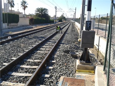
In order to assess the different computational considerations of the 3-D FEM model, real vibration data from an existing track have been measured. This track is located in the Line 1 of the Alicante Tram network and the stretch is located between Campello and Poble Espanyol stations. In the next paragraph a description of the elements that have to be included in the model is done.
Fig. 1Overview of the measured track
It is a straight section of a double track ballasted track comprised of UIC54 rails and single-block DW sleepers. Distance between adjacent sleepers is 0.6 m and an elastomeric railpad is located between the rail and the sleeper. The thickness of the ballast layer is 0.2 m (measured from the bottom of the sleeper) and this layer rests directly on the ground. Mechanical properties of the ground are unknown and will be determined in the calibration process. In the next table, the mechanical properties of the rest of the track elements are displayed. Unknown parameters, which are represented by a dash, will be determined in the calibration process.
Table 1Mechanical properties of track elements
(Pa) | (kg/m3) | ||
Rail | 2.1×10¹¹ | 0.3 | 7850 |
Railpad | 178.57×10⁶ | 0.3 | 900 |
Sleeper | 2.7×10¹⁰ | 0.25 | 2400 |
Ballast | – | 0.3 | 1900 |
Ground | – | 0.3 | 2000 |
The vehicle driving along the track is a Vossloh 4100 train at a speed of 35.2 km/h. Each train is composed by three units: two top carriages and one placed in between and the transmitted load per axle is 100 kN. Given the symmetry of the problem around the middle-track longitudinal axis in the calculations, it is only considered the load transmitted by a wheel which, for each one of them, is 50 kN.
In the real data acquisition campaign Sequoia Fast Tracer™ three-axial accelerometers were used. The device used to validate the model was located on the sleeper, 0.3 m away from the external side of the rail while data used to calibrate the model were collected using an accelerometer located on the rail foot. The properties of the accelerometers used are shown in Table 2.
Table 2Properties of Sequoia Fast Tracer accelerometers used in the data acquisition campaign
Sensors on rail and sleeper | |
Scope | ±5 g |
Bandwidth (Hz) | 0-2500 |
Resolution (m/s2) | 0.041 |
Noise (m/s2) | 0.075 |
Sampling rate (Hz) | 8192 |
3. Three-dimensional finite element model
The 3D Finite Element Method software used to perform the numerical model is ANSYS PRODUCT LAUNCHER V.11. The proposed dynamic problem is based on solving the equilibrium between internal and external forces given by Eq. (1):
where is the global mass matrix, is the damping matrix, is the stiffness matrix, is the vector of displacements, is the vector of velocities and is the vector of accelerations. In the other side of the equation, the time-dependent external forces vector appears.
Rayleigh damping theory used in the model includes a damping matrix which can be calculated as is shown in Eq. (2):
here and are the Rayleigh coefficients, needed to solve the dynamic analysis and and are the mass and stiffness matrix respectively. If an orthogonal transformation of Eq. (2) is done as in Real et al. [8] the damping matrix turns into a diagonal matrix where the value of the -th element in the matrix is given by the following expression in which is the -natural modal frequency of the system:
Furthermore, considering the hypothesis of the analogy to single-degree-of-freedom systems, the elements can be calculated from:
By comparing Eq. (3) and Eq. (4) and isolating the term the next relationship can be established:
The contribution of the term decreases as the natural modal frequency increases. For this reason, in case of structures with high stiffness, which means high values of natural modal frequencies, this term is often neglected considering the single contribution of the second part of the identity:
Consequently, the mass contribution to the damping drops form Eq. (2) and the damping matrix to be introduced in Eq. (1) is given by:
3.1. Model scheme
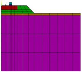
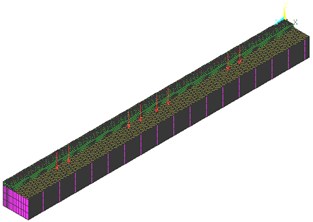
Fig. 2 shows the symmetrical cross-section of the model. It can be seen in a descending order the rail and the railpad over the sleeper resting on the ballast layer which is displayed in green. Underneath the ballast layer, the ground is located. The ground is represented by elements of different colors; it is only related to the depth of the elements but the mechanical properties of the brown elements and the purple elements are exactly the same. Properties described in Table 1 are assigned to the different elements in Fig. 2.
Fig. 2Model scheme
In order to achieve a simplified representation of the rail in the model that allows meshing this element, the rail has been represented by a rectangular prism with a contact surface with the railpad equal to the width of the original rail foot. Moreover, the inertia must be equal to that of the original rail and consequently, the height of the prism in the model is conditioned by this inertia. Thus, the stress transmitted to the railpad by the rail and the bending mechanism will be exactly the same as in reality. This simplification has been already done by Real et al. [13] and the quality of the results was not affected. Analogously, railpad Young modulus in Table 1was obtained from the real vertical stiffness of the material, taking into account the size of the element which accounts for the railpad in the model. It can be done equaling the real vertical stiffness to the model vertical stiffness with the following equation:
It is known that the real vertical stiffness of the model is 100 kN/m; the height of the railpad in the model is 0.05 m and the element area is 0.28 cm2. Subsequently, the term in Table 1 is obtained from Eq. (9) and then introduced as an input of the FEM model.
3.2. Model and elements size
Model dimensions are determined by the frequency range intended to study. Although vibrations induced by a passing train comprises a wide range of frequencies, Griffin [14] pointed the interval from 2 to 50 Hz as the most important from the approach of the negative effects on people. This statement was considered by Kourioussis et al. [15] to establish an upper frequency threshold in the study of the vibration effects on buildings and people located in the railway surroundings.
As well as the frequency range, it is important to know the Rayleigh waves speed in the ground. This speed can be considered a 10 % lower than the P-waves speed of the ground and therefore it is calculated with the following equation:
Since the elastic modulus of the ground is an unknown parameter, a typical value of 120 MPa for this type of soil is assumed. Rest of the properties are taken from Table 1 obtaining a value for the Rayleigh wave speed of 137 m/s.
From the speed, the maximum wavelength which determines the length and the width of the FEM model can be obtained using Eq. (10):
This equation yields for and a maximum wavelength . Analogously, the minimum wavelength corresponds to the highest frequency of study and it is calculated with the following equation:
From which a minimum wavelenght of is obtained for a maximum frequency of . According to Andersen and Jones [16], in this minimum wavelength at least 6 nodes must be inscribed. Consequently, the maximum dimension of the elements’ edge in the model is calculated with Eq. (12) and results in :
The previous meshing criteria have been already used in 3D FEM methods obtaining high quality results for the vibration phenomenon in [8] and [13].
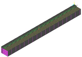
Since the sleeper width, measured in the track longitudinal direction, is 20 cm, an element size of 10 cm is chosen. This figure is in complete agreement with the previous meshing restrictions and this element size also allows applying the load in the node situated in the middle of the sleepers, which are separed 0.6 m from each other.
3.3. Load application
The form in which loads are implemented in the model is discussed in section 4. However, it is necessary to validate the model as a previous step to the computational considerations discussion. For this reason, the response to a single axle load is calculated expanding then the solution by adding together these single responses to account for the whole train as in [8]. To calculate this response, the train speed and the configuration of the axles in the vehicle displayed in Fig. 3 are needed. With the previous parameters, the time instant in which each load is transmitted by each pair of wheels can be determined. In Fig. 4 the red arrow represents the load whose modulus depends on the train weight being in this case 50 kN.
Fig. 3Axle distribution in the top vehicles (upper) and in the intermediate vehicle (lower)
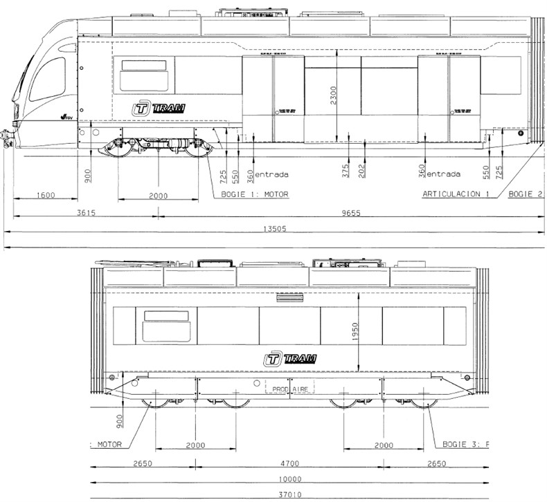
Fig. 4Single wheel load effect represented in the 3D FEM model
3.4. Sensitivity analysis
The aim of the sensitivity analysis is to assess the influence of the different model inputs on the final results. Since some mechanical parameters of the ballast and the ground are unknown, their influence on the final vibration results must be obtained. In order to perform it, random values are chosen for the Young modulus, Poisson ratio and global damping coefficient which accounts for both ballast and ground. Values chosen must be coherent from the engineering point of view and it is recomended to take values from pevious experiences as [8]. By modifying the value of the parameters and analyzing the response of the model against changes, significant parameters of the model can be identified and then determined in the coming process of calibration.
Rayleigh global damping coefficient and Young moduli for the ballast layer and the ground have been found of strong influence on the model response. Thus, these significant parameters will be calibrated in the next step.
3.5. Calibration and validation of the model
From the previous sensitivity analysis, it is concluded that three parameters need to be calibrated: Rayleigh global damping coefficient, Young modulus of the ballast and Young modulus of the ground. To perform the calibration, different combinations of values for these three parameters are proposed; being the combination which presents more accuracy in the results when compared to real data the chosen to establish the computational considerations in section 4.
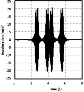
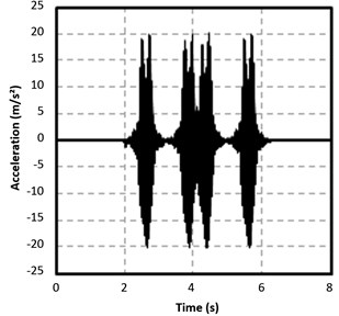
Fig. 5Accelerations on the sleeper. Validation of the 3D FEM model
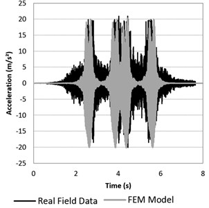
Data set chosen to calibrate the unknown significant parameters was measured in the rail foot. Using the results obtained in the calibration, the vibrations on the sleeper at a point located 50 cm away from the outer side of the rail were calculated and then compared with another set of real measured data. This comparison between calculated and measured data on the sleeper was done in order to validate the model. Results are displayed in Fig. 5.
In Fig. 5 it is appreciated that the acceleration peaks corresponding to the axle load transmitted are similar in magnitude in both graphics. In addition, maximum and minimum peaks calculated as well as the timing of the peaks faithfully represent the real response. These validation criteria based on morphological features of the measured and calculated accelerograms has been already used in [8], resulting exhaustive enough for the purpose of this paper devoted to computational considerations.
The values of the unknown parameters which were found significant in the sensitivity analysis are presented in Table 3. These values, in addition to those defined in Table 1, are the inputs of the different scenarios defined to assess the computational considerations in the next section.
Table 3Calibration values
Parameters | Calibrated values |
Rayleigh coefficient | 0.0005 |
Ballast Young modulus | 15 MPa |
Subgrade Young modulus | 120 MPa |
4. Computational considerations
A comprehensive methodology addressed to train-induced vibration study has been presented in the previous sections. In this part, the influence of four main aspects of the method is discussed. These considered aspects are: how loads are applied; which calculation element is used; the elements size in the mesh and reflections about the constitutive models of the materials in the model.
In the four analyses presented, different alternatives are compared attending to the quality of the results obtained as well as to the computation time required in each case. All the scenarios are calculated using a PC with a processor IntelCore™ i7-3820 of 3.6 GHz and an installed RAM memory of 32 GB. In this manner it is discussed if the quality of the results justifies the computational extra cost.
4.1. Load application
In this section two different forms to apply the load are presented. A priori, it can be asserted that calculation time and the results obtained will be different as a consequence of the different assumptions considered.
The first form considers a single load whose modulus corresponds to the load transmitted per axis by the train. After calculating the vibration response that the single load produces in the track, the superposition principle is applied. In this manner it is calculated the whole train response as the summation of the individual axle response. The effect that each axle produces on the track is identical but presenting a time delay. For this reason it is necessary to know the axle distribution in the vehicle (Fig. 3) and the train speed; both determine the time instant in which each axle appears. This procedure is identical to that used in section 3 to calibrate and validate the model and it has been also previously used by authors such as El Kacimi et al. [17] who simulated the response of a whole train from the individual response of a vehicle composed of two bogies. In the same manner, Lu et al. [18] studied the response of a train modeling the load as moving masses over the axles which appear as the train moves along the structure.
Another form of introducing the loads in the model is to directly consider the complete train. This method was followed by Ekevid and Wiberg [19] to analyze the wave propagation in high speed lines using a scaled boundaries FEM method as an alternative to the traditional FEM method. Hall [20] also used this load implementation method to calculate vibrations in the track elements using a 3D FEM method as well as Zhai and Song [21] to estimate vibrations induced by moving loads with a moving coordinate system. All the previous examples consider that all the axles are simultaneously acting and therefore it is not needed to apply the superposition principle. The scheme corresponding to this loading case is shown in Fig. 6.
Fig. 6Whole train load effect represented in the 3D FEM model
Both simulations have been run with an element SOLID45 with 10 cm edge. Results obtained are displayed in Fig. 7.
Fig. 7Comparison of results: superposition principle a) and whole train b)

a)
b)
Results obtained using both methods are almost identical. The shape of the accelerogram, the time distribution of the peaks and the characteristic maximum and minimum values are the same. For these reasons it is concluded that the results are independent to the form used to implement the loads in the model.
Table 4Computing time for different input load methods
Input load | Computing time |
Single-axle Response + Superposition | 2 hours 50 minutes |
Whole train | 4 hours 52 minutes |
In Table 4, computing time is shown for each loading case. It can be seen a calculation time reduction of more than a 40 % in the case of considering the single load effect and then applying the superposition principle. From this fact, added to the similarity of the results obtained using both methods, it is concluded that the direct consideration of the whole train is an inefficient alternative from the computing point of view. Moreover, in this case, the vehicle only has 8 axles; it leads to the conclusion that in vehicles with more axles single load consideration would be even more suitable.
4.2. Type of element
The influence of the type of element used in the model meshing is studied here. In each model, the element chosen must yield good results in the case of displacements, vibrations and accelerations. As a first approach, it may be thought that the number of nodes per element and the degrees of freedom assigned to them have influence on the final results. The effect of the number of nodes per element was studied by Wood et al. [22] in a FEM model which represented a human cranium. From this study both stress and displacement fields were obtained using elements of 4 and 10 nodes, obtaining results with slight differences. In the case of this paper, this consideration is done in a much wider dominium in which elements are rectangular prisms with edge lengths larger than in the previous case.
Being that hexahedral elements have been traditionally used to model three-dimensional forms when working with ANSYSv11, it is presented below the influence on the results obtained when considering two different types of “SOLID” elements: SOLID45 and SOLID95.
Fig. 8SOLID95 a) and SOLID45 b) elements
a)
b)
SOLID45 element includes 8 nodes located in the hexahedral vertices. Each one of these nodes has three degrees of freedom corresponding to the three dimensional space translations. On the other hand, the SOLID95 element adds extra nodes on each of the middle points of the edges with regard to the previous element. Consequently, this element has 20 nodes with the same degrees of freedom and therefore results are expected to be closer to the real vibration response of the system.
The 8-nodes elements have been widely used to calculate vehicle-induced vibrations. Some examples are found in previous researches made by Hall [20] in the case of railway induced vibrations and by Ju [10] for truck induced vibrations.
Fig. 9Comparison of results: SOLID45 a) and SOLID95 b)
a)

b)
As shown in Fig. 9, results are very similar for both elements. The rest of variables have been set equal: 10 cm edge for the element and superposition principle application starting from the single load response. The shape of the accelerogram does not depend on the element type as well as the timing of the peaks. However, some differences of around 1.5 m/s2 in the positive peak values and of around 2.5 m/s2 in the negative peaks are observed. In both cases the accelerations are slightly higher in the case of using the SOLID95 element. These minor differences in the peak values could be corrected in a new calibration process by diminishing, for instance, the value of the damping coefficient or increasing the Young moduli of the ballast and the ground. These changes are addressed to obtain lower acceleration values which represent more faithfully the real phenomenon.
However, each scenario in this new calibration process would require three times as much computational effort as in the SOLID45 case according to Table 5. This extra time consumption would not be justified since results obtained with the 8-nodes element match accurately the real registers. In short, the inclusion of extra nodes brings with a significant increase in computing time. A change from an 8-nodes element to another with 20 nodes triples the calculation time and, comparing the results obtained using both elements, this change is not efficient from the computational viewpoint.
Table 5Comparison of computing time for the consideration different elements
Element type | Computing time |
SOLID45 | 2 hours 50 minutes |
SOLID95 | 8 hours 34 minutes |
4.3. Elements size
This subsection deals with the element dimension and its influence on the quality of the results. This fact was studied by Fischer [23] in a machinery cutting process of small steel elements. Results concluded that the element size determines the quality of the results. Model was 1 mm length and the length of the elements chosen was 0.04 mm which means 25 times smaller. The vibration case studied in this paper has a model dimension of 70 m and the element lengths studied are 0.01 m and 0.005 m what supposes a ratio between the length of the element and the length of the model of 1:700 and 1:1400 respectively; in any case, very different from those obtained in the previous study.
For railway induced vibrations modeling, Hall [20] used an element length of 0.65 m in the track structure layers and the upper part of the soil. This length was steadily increased up to 8 m in the deeper layers. In the case of this paper, element size is constrained by the wave considerations presented in section 3.2.
Fig. 10Comparison of results: 5 cm meshing a) and 10 cm meshing b)
a)

b)
Results obtained in two scenarios for which the element size varies are displayed in Fig. 10. Calculations have been done considering again the superposition principle and using the element SOLID45. Both graphs are similar since the time distribution of the peaks in the accelerogram is exactly the same and the value of the maximum accelerations as well. In addition, in Fig. 10(a) the body of the accelerograms is more filled as a consequence of using a denser mesh. However, in this same graph, corresponding to the 5 cm element edge, it is seen how the lower peaks lightly differ from the real values. This effect might suggest, as in the previous case when the type of element was studied, that the previous calibration and validation process should be repeated as a result of changing the element size in order to adjust the small differences existing.
With regard to the computation time, it is deduced from Table 6 that when using a denser meshing, the time significantly ascends. Calculation time increases and the possible need of a new calibration and validation process, in which each proof would consume the time indicated in the table below, leads to the consideration that a size of 5 cm for the edges of the hexahedral elements is not efficient given the accuracy obtained when using a 10 cm-edge element.
Table 6Comparison of computing time for the consideration different elements
Element size | Computing time |
10 cm | 2 hours 50 minutes |
5 cm | 7 hours 44 minutes |
4.4. Constitutive model of the materials
The main objective of this section is to determine if the linear elastic assumption for the materials included in the track structure is appropriated in this case or if would be convenient to use other constitutive models for any of the materials. To do so, stresses are calculated in all the materials across the track cross section using the same model as in the vibration study. The only difference is the output desired, which in this case is the stress level instead of the accelerations. By comparing the stresses with the stress threshold above which the linear elastic behavior of the material is not ensured, the suitability of this simplification is assessed. Additionally, it must be highlighted that one of the conditions to apply the superposition principle is the linearity and if this requirement is not satisfied, the single-load effect consideration explained in 4.1 would be useless.
Ballast layer is excluded from this analysis since the stress field obtained from the model does not precisely represent the real behavior of the ballast particle. In reality, contacts between these particles are discrete and not continuous as in the model. Thus, the real stresses suffered are higher due to the lower contact surface. Ergenzinger et al. [24] formulated a 3D FEM model that represents each ballast particle separately and analyzed the influence of the transmitted stress on the number of discrete contacts broken. In a model like this, it would be possible to study the stress-strain relation in the ballast.
The maximum vertical stress transmitted over the ground by the ballast layer is only 6.5 kPa. This figure, compared to those in Table 7, reveals the effectiveness of the ballast layer in the load distribution and the consequent stress decrease. Considering a high quality and properly compacted ground, the low tension experienced would induce negligible displacements and the linear elastic model could be perfectly assumed without compromising the results.
Table 7Maximum stresses in the track elements (MPa)
Rail | 29 |
Railpad | 0.67 |
Sleeper | 1.12 |
On the other hand, elements located over the ballast layer suffer the higher stresses in the track. It is due to the fact that these elements transfer all the force transmitted by the vehicle, being the contact surfaces between them very reduced. In the following table the maximum stresses in rail, railpad and sleeper are shown according to Von Mises criterion.
From Table 7 it is deduced that the rail does not reach the steel yielding strength under the given loads. In agreement to Ahlström and Karlsson [25] the maximum stress in the rail is also far from the minimum fatigue stress fixed in 460 MPa to 10.000 load cycles. For both reasons it would not be adequate another constitutive model for the steel distinct from the linear elastic in this case.
In the case of the concrete sleepers, it exist a phenomenon that modifies the linear elastic behavior of the material which is produced in a stress level lower than the yielding: the cracking. Cracking stress of a prestressed concrete due to tensile stress is around 3 MPa [26]. As the maximum stress in the sleeper is 1.12 MPa it can be asserted that the linear elastic model results also suitable for this element.
Regarding the railpads, it must be pointed the effect that cyclic loads have on elastic railpads. This influence was studied by Carrascal et al. [27] and it was determined that high values of humidity or extreme temperatures may modify the elastic behavior of the material. Considering that the studied railway stretch is located in Alicante and this region is characterized by a dry climate zone with mild temperatures, an ideal linear behavior is expected for the railpads. Therefore, the material constitutive model chosen for this element is justified.
On the basis of the previous discussion, the need of performing a stress analysis of the structure to calculate the stresses in each one of the material is needed. It must be done in order to demonstrate that the strain-stress model previously assigned to any of the materials is correct.
Dynamic overloads induced in high speed lines or huge loads transmitted by freight trains in different cases from this may cause that the materials behavior moves away from the linear elastic. Consequently, the most suitable constitutive model for the different materials of the track must be carefully selected taking into consideration the conclusions deduced from the previous stress study.
5. Conclusions
From the results obtained from the previous scenarios, the following conclusions can be drawn:
1) The vibration response is not altered by the form in which loads that cause it are implemented. Obtained results are identical if a single axle effect is calculated and then extended according to the superposition principle and if the whole train effect is directly calculated. However, the first alternative is more efficient from the computational point of view and thus, preferable if the linear behavior of the materials is ensured.
2) The analysis using elements with more nodes or a smaller edge length markedly increases the computation time. Additionally, these modifications may require new calibration and validation processes of the model with the consequent computation time increase. If results obtained with the first approach are accurate enough, it is recommended neither considering more nodes per element nor reducing the elements’ edge length.
3) The linear elastic behavior assumptions of the materials must be duly justified by a stain-stress study of the railway structure. Although in the case analyzed in this paper stresses are in agreement to the linear elastic behavior, in other tracks with different conditions might not be true. Special attention should be paid to high speed lines and freight lines since dynamic overloads or huge loads transmitted per axle may respectively affect to the linear behavior of the materials. If this happens, superposition principle used to calculate the whole train response from the single axle response would be useless.
Previous conclusions have been obtained from a 3D FEM model calibrated and validated in a real track using a computer with given characteristics. However, results obtained can be perfectly extrapolated to different simulation models based on the Finite Elements Method.
References
-
Dawn T. M., Stanworth C. G. Ground vibrations from passing trains. Journal of Sound and Vibration, Vol. 66, Issue 3, 1979, p. 355-362.
-
Degrande G., Schillemans L. Free field vibrations during the passage of a Thalys HST at variable speed. Journal of Sound and Vibration, Vol. 247, Issue 1, 2001, p. 131-144.
-
Krylov V., Dawson A., Heelis M., Collop A. C. Rail movement and ground waves caused by high-speed trains approaching track-soil critical velocities. Journal of Rail and Rapid Transit, Vol. 214, Issue 2, 2000, p. 107-116.
-
Madshus C., Kaynia A. M. High-speed railway lines on soft ground: dynamic behaviour at critical train speed. Journal of Sound and Vibration, Vol. 231, Issue 3, 2000, p. 689-701.
-
Forrest J. A., Hunt H. A three-dimensional tunnel model for calculation of train-induced ground vibration. Journal of Sound and Vibration, Vol. 294, Issue 4, 2006, p. 678-705.
-
Auersch L. The excitation of ground vibration by rail traffic: theory of vehicle-track-soil interaction and measurements on high-speed lines. Journal of Sound and Vibration, Vol. 284, Issue 1-2, 2005, p. 103-132.
-
Galvín P., Domínguez J. Experimental and numerical analyses of vibrations induced by high-speed trins on the Córdoba-Málaga line. Soil Dynamics and Earthquake Engineering, Vol. 29, Issue 4, 2009, p. 641-657.
-
Real J. I., Galisteo A., Real T., Zamorano C. Study of wave barriers design for the mitigation of railway ground vibrations. Journal of Vibroengineering, Vol. 14, Issue 1, 2012, p. 408-422.
-
Hatzigeorgiou G., Beskos D. Soil-structure interaction effects on seismic inelastic analysis of 3D tunnels. Soil Dynamics and Earthquake Engineering, Vol. 30, 2010, p. 851-861.
-
Ju S. Finite element investigation of traffic induced vibrations. Journal of Sound and Vibration, Vol. 321, Issue 3, 2009, p. 837-853.
-
Kouroussis G., Verlinden O. Prediction of railway induced ground vibration through multibody and finite element modelling. Mechanical Sciences, Vol. 4, Issue 1, 2013, p. 167-183.
-
Kouroussis G., Verlinden O., Conti C. On the interest of integrating vehicle dynamics for the ground propagation of vibrations: The case of urban railway traffic. International Journal of Vehicle Mechanics and Mobility, Vol. 48, Issue 12, 2010, p. 1553-1571.
-
Real J. I., Galisteo A., Asensio T., Montalbán C. Study of railway ground vibrations caused by rail corrugation and wheel flat. Journal of Vibroengineering, Vol. 14, Issue 4, 2012, p. 1724-1733.
-
Griffin M. Handbook of Human Vibration. Academic Press, USA, 1996.
-
Kourioussis G., Verlinden O., Conti C. A two-step time simulation of ground vibrations induced by the railway traffic. Journal of Mechanical Engineering Science, Vol. 226, Issue 2, 2012, p. 454-472.
-
Andersen L., Jones C. J. C. Three-Dimensional Elastodynamic Analysis Using Multiple Boundary Element Domains. ISVR Technical Memorandum, University of Southampton, 2001.
-
El Kacimi A., Woodward P., Laghrouche O., Medero G. Time domain 3D finite modelling of train-induced vibration at high speed. Computers and Structures, Vol. 118, Issue 8, 2013, p. 66-73.
-
Lu Y., Mao L., Woodward P. Frequency characteristics of railway bridge response to moving trains with consideration of train mass. Engineering Structures, Vol. 42, 2012, p. 9-22.
-
Ekevid T., Wiberg N. Wave propagation related to high-speed train. A scaled boundary FE approach for unbounded domains. Computer Methods in Applied Mechanics and Engineering, Vol. 191, Issue 36, 2002, p. 3947-3964.
-
Hall L. Simulations an analyses of train-induced ground vibrations in finite element models. Soil Dynamics and Earthquake Engineering, Vol. 23, Issue 5, 2002, p. 403-413.
-
Zhai W., Song E. Three dimensional FEM of moving coordinates for the analysis of the transient vibrations due to moving loads. Computer and Geotechnics, Vol. 37, Issue 1, 2009, p. 164-174.
-
Wood S., Strait D., Dumont E., Ross C., Grosse I. The effects of modelling simplifications on craneofacial finite element models: The alveoli (tooth sockets) and periodontal ligaments. Journal of Biomechanics, Vol. 44, Issue 10, 2011, p. 1831-1838.
-
Fischer C. Runtime and accuracy issues in three-dimensional finite element simulation of machining. International Journal of Machining and Machinability of Materials, Vol. 6, Issue 1-2, 2009, p. 35-42.
-
Ergenzinger C., Seifried R., Eberhard P. A discrete element model for degradation of ballast tracks. Proceedings in Applied Mathematics and Mechanics, Vol. 12, Issue 1, 2012, p. 49-50.
-
Ahlström J., Karlsson B. Fatigue behaviour of rail steel-a comparison between strain and stress controlled loading. Wear, Vol. 258, Issue 7, p. 1187-1193.
-
Ramennikov A. M., Murray M. H., Kaewunruen S. Reliability-based conversion of a structural design code for railway prestressed concrete sleepers. Journal of Rail and Rapid Transit, Vol. 226, Issue 2, 2011, p. 155-173.
-
Carrascal I., Casado J., Polanco J., Gutiérrez-Solana F. Dynamic behavior of the railpads in railways. Annals of Fracture Mechanics, Vol. 22, 2005, p. 372-377, (in Spanish).
About this article

