Abstract
To investigate the inherent complex dynamic characteristics of luffing mechanism of auger driller, the rigid body motion of structures and the dynamic behavior of the drive system should be studied in an integrated model. The working principle and structural characteristics of the luffing mechanism is firstly analyzed, then the bond graph model of revolute joint, cylinder and boom are proposed based multi-body theory, and the bond graph model of hydraulic system is also constructed. Through the analysis of the dynamic characteristics and interaction rules of each sub model, the transmission path of power flow is described. Coupling the boom structure and hydraulic actuator, the complete bond graph model of luffing mechafnism have been developed in a unified way. The total governing equations of the system have been derived from the model. Numerical results of chamber pressure of luffing cylinder implies to the good accuracy of the bond graph study, while comparing with experimental results. Meanwhile, the effects of the installation position parameters of the joints on system response have been studied through simulation, which provides a theoretical basis for improving the dynamic performance of the luffing mechanism.
1. Introduction
Auger driller is widely used in pile foundation construction for the advantages of low noise, less pollution, high efficiency and less operators in the working process. Auger driller is mainly composed of boom, hydraulic dynamic head, slewing platform, luffing mechanism and longitudinal movement mechanism. The luffing mechanism is an important working equipment used for supporting the boom and changing its amplitude, whose dynamic performance has a significant influence on the key performance indexes of the auger driller, such as the constraint force of the revolute joint, the chamber pressure of luffing cylinder, the maximum output torque of hydraulic dynamic head and so on. The dynamic performance of the luffing mechanism varies with its different structure.
Many studies on the luffing mechanism have been reported in the literature, but the existing published articles mainly concentrated on its unilateral features. Kang [1], Yang [2] and Wang [3] investigated the dynamic characteristics of the system during luffing motion using multi-body dynamics theory. The boom is driven by luffing cylinder, which has a prescribed velocity, but the method of “kinematic forcing” with the assumed profiles of the driving velocity could not accurately describe the driving output of the hydraulic actuator, especially at the time of start-up and braking of the system. Xu [4] proposed a new optimization method for portal cranes’ luffing system design based on the hybrid neural networks. Lin [5] studied the synthetical genetics annealing for the trajectory optimization of the luffing mechanism. He [13] and Zhu [14] focused on the analysis for the strength of component. Yi [15] and Zhu [16] researched the load characteristics of luffing cylinder. Wang [17] demonstrated the effects of throttle valve of the return oil circuit and counterbalance valve on the vibration of the boom when declining, but the boom is simplified as a mass in their study, which leads to an imprecise description of boom motion. The model of the boom is coupled with the model of hydraulic system during luffing process, so the motion of the boom and the dynamic behavior of the hydraulic system should be studied with one integrated model. However, little research of the integrated modeling method for simulating the luffing dynamic behavior is done.
The method based on analytical mechanics and theory of elasticity is limited to mechanical energy domain, failed to unify the physical quantity in different energy domain, so the application of the model is restricted to a certain extent [1-3]. Consequently, other analytical approach such as bond graph method based on energy and information flow is considered to be more desirable in the present study. It is a power tool for modeling complex system even with interaction of several energy domains. A complete bond graph model of the luffing system explaining the physical characteristics of each element is developed, then the system state equations have been derived algorithmically in a systematic manner from the model. In continuation, the effects of the install position parameters of the joints on system response are investigated. Also, this modeling method is verified experimentally.
2. Multi-body dynamic model for luffing mechanism
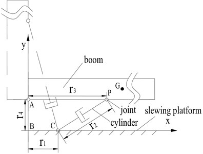
As shown in Fig. 1, the luffing mechanism of auger driller is composed of luffing cylinder, slewing platform and boom. They are connected to form a crank and rocker mechanism through revolute joints (A, C, P). The cylinder motivated by hydraulic oil supplied from the pump pushes the boom to rotate around the joint A from the horizontal position to the vertical position. The inertial coordinate system is set up on the slewing platform, for it is fixed on the ground during luffing motion. To simplify the simulation, the mechanical part of the luffing mechanism is divided into three subsystems, including revolute joint, boom and luffing cylinder. The bond graph model for each subsystem is constructed, and then the complete multi-boy dynamic bond graph model of luffing mechanism is made.
Fig. 1Schema for luffing mechanism
2.1. The model of revolute joint
The revolute joint is one of the basic components of planar mechanisms. As shown in Fig. 2, the rigid links are connected by the revolute joint. The clearance between the bearing and journal is necessary to reduce friction and ensure the smooth motion. Specially, when the heat generated by the rotating friction heat makes journal expands unceasingly, the interference fit between the bearing and shaft can be avoided by a certain gap. But on the other hand, joint clearance often results in rapid wear, impact forces, rattling and noise. There are two directions of force between the bearing and journal, named normal force and tangential force, respectively. The normal force acts along the attitude line, and the tangential force acts perpendicular to attitude line. Various authors have constructed various formulations for these forces. In the present study, the flexible joint without clearance is taken as the object of study. In order to simply the simulation, the dry-friction is omitted and viscous friction is considered. Consequently, the tangential force is equal to zero and the interaction force between the bearing and the journal in - reference frame can be calculated as:
where . , are the absolute coordinates of the center of the bearing and journal, respectively. The effective stiffness can be computed experimentally or numerically, e.g., from a finite element model. The damping is proportional to the effective stiffness.
In order to facilitate the expression of the bond graph model, Eq. (1) can be expressed as:
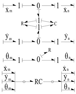
As shown in Fig. 3, the bond graph model of the revolute clearance joint has been developed. The constraint force of the revolute joint can be calculated by the R and C elements. The model can also be represented in a compact form using RC field element and vector bonds, as show in the bottom of Fig. 3.
Fig. 2Schema for revolute joint
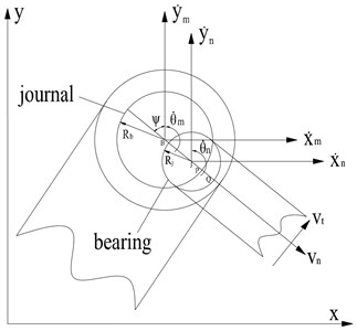
Fig. 3The bond graph model of revolute joint
2.2. The model of the boom
Fig. 4Schema for boom
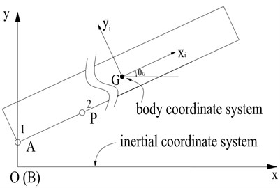
The boom can be considered as rigid link due to its large bending stiffness. As shown in Fig. 4, the body fixed frame is used on the rigid link, is set along the axial direction of the boom. If the coordinate of the gravity of the boom and the angular position of the body fixed frame relative to the inertial frame about -axis, according to the law of transformation between body coordinates and inertial coordinates, the absolute coordinates of any point on the boom can be described as:
where and are the coordinates of point in the body fixed frame. and are the coordinates of center of gravity.
Differentiating Eq. (3) with respect to time, Eq. (4) can be obtained as follow:
Using the following definitions: and , Eq. (4) can be rewritten as:
Eqs. (3) and (5) are sufficient to develop the bond graph model of the boom as shown in Fig. 5. This model only includes two revolute joint, but it is easy to add the number of joint based the actual structural of rigid link. The boom can be linked with other components by the revolute joint. In Fig. 5, the moment of inertia and the mass can be modeled by I elements connected with the 1 junction representing the velocities of the mass center of the boom in the inertial frame. A bond with a circle over it represents a vector bond and a thick vertical line is used to split a vector into scalar bonds or to merge scalar bonds to form a vector bond. The force and torque can be considered as effort sources and added to the corresponding 1-junctions. For example, the effort source SE: is added to the 1 () junction, which represents the gravity of the boom.
Fig. 5The bond graph model of boom
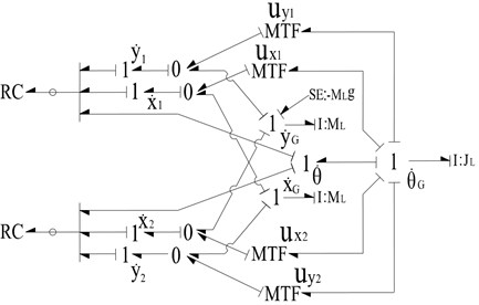
According to the flow vector relationship across the transformer (Eq. (5)), the force and moment balance equations can be derived from the model as follow:
where and represent the forces of joint in and direction. and represent the forces of the center of gravity in the and direction. represents the torque of the center of gravity along the axis. The dynamic equations describing the boom can be derived by the Newton – Euler theory, which is the same as Eq. (6). Therefore, the bond graph model in Fig. 5 is correct.
2.3. The model of the cylinder
The slider is one of the most difficult problems of multi-body dynamic analysis. The cylinder is a typical slider, which is widely used in the hydraulic system of engineering machinery. The schematic view of the cylinder is shown in Fig. 6, which is mainly composed of cylinder and piston rod.
According to the law of movement of cylinder, the velocities of the end points C and P can be expressed as:
where and represent the angles of cylinder and piston rod relative to the inertial frame, the meaning of geometric parameters in the above equations is shown in Fig. 6.
Fig. 6Schema for the cylinder
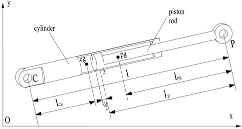
Differentiating the length () between the points C and P may be written as:
The normal velocity at the contact point 1 on the cylinder and the piston can be described as:
To calculate the reaction force of contact point, the fictitious compliance and resistance elements are added to the corresponding 1-junction, which is verified by Bera [9].
The normal velocity at the contact point 2 on the cylinder and the piston can be described as:
Likewise, the reaction force of contact point 2 can be computed by the same method.
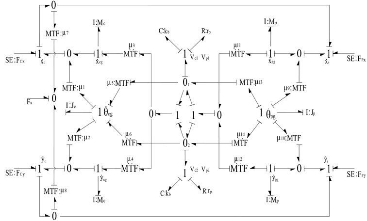
The bond graph model of cylinder has been developed based on Eqs. (7)-(15) as shown in Fig. 7. The compliance and resistance elements all have integral causality. The different multipliers used as MTF mlduli in the model are. In Fig. 7, the effort sources represent the constraint force of joint C and P. The 1-junctions indicate the various velocity points, the I elements are used to model the mass and the moment of inertias of the cylinder and the piston rod, respectively. The relative velocity between the cylinder and the piston rod can be calculated by by MTF elements with moduli and connecting to the 0-junction. The force acting on the piston also can be modeled by this junction. represent the damping coefficient of the relative motion between the cylinder and the piston rod. and are the effective stiffness and damping coefficient of the contact points.
Fig. 7The bond graph model of cylinder
3. Model of hydraulic system of luffing mechanism
The hydraulic system of luffing mechanism is shown in Fig. 8. A constant flow pump, driven by an electric motor, supplies hydraulic power to the cylinder. The cylinder is subjected to the gravity and inertial of the boom. To prevent the boom from overrunning or counter the weight of the boom, the counterbalance valve is placed. The four way, three position electro-hydraulic direction control valve is used to control the telescopic action of the cylinder, when the boom reach the target position, it is fully closed immediately. In the development of the dynamic model of this hydraulic system, the following assumptions are made: (a) capacitive effects or resistive effects are lumped wherever appropriate; (b) the pump discharges the fluid steadily, the flow ripples is also ignored for simplification; (c) responses of the counterbalance valve and the unloading valve are instantaneous; (d) the speed of the electric motor is constant. Finally, as shown in Fig. 9, the complete bond graph model of the hydraulic system during luffing motion has been constructed.
Fig. 8Hydraulic system of luffing mechanism (1 – constant flow pump, 2 – unloading valve, 3 – pipe 1, 4 – pipe 6, 5 – oil filter, 6 – directional control valve, 7 – pipe 2, 8 – pipe 5, 9 – counterbanlance valve, 10 – pipe 3, 11 – pipe 4, 12 – luffing cylinder)
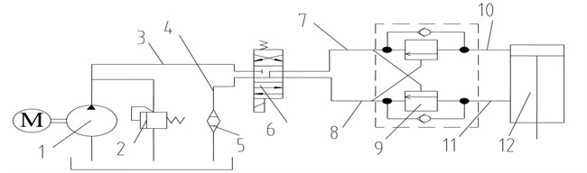
Fig. 9The bond graph model of the hydraulic system during luffing motion
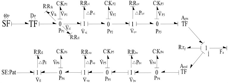
In the above model, the flow source SF element is the speed of the constant flow pump. The moluli represents the displacement of the pump. The element indicates the leakage resistance of the pump. , , , , and are the equivalent hydraulic stiffness of the corresponding chambers. The unloading relief valve resistance is indicated by element, through which the flow goes to the tank when the system pressure exceeds the setting pressure of the valve. The flow and to the inlet and outlet port of the direction control valve depend on the port resistance and , which are controlled by its opening area. The integral check valve is considered as element, through which the flow depends on the differential pressure across it. The element represents the resistance of counterbalance valve, the flow passes to the cylinder. The transformer modulus and are the cap side area and rod side area. The flow through the filter element causes a pressure drop due to its resistance .
The system equations derived from the model are as follows:
The volume rate of change of the fluid in pipe 1 is given by:
where , , .
The volume rate of change of the fluid in pipe 2 is given by:
where .
The volume rate of change of the fluid in pipe 3 is given by:
Referring to Fig. 9, the force equilibrium equation of the piston is calculated by:
The volume rate of change of the fluid in pipe 4 is given by:
where .
The volume rate of change of the fluid in pipe 5 is given by:
where .
The volume rate of change of the fluid in pipe 6 is given by:
where .
The pressures at different pipes can be calculated by:
where 1, 2,…,6, is the serial number of the pipes as shown in Fig. 8.
4. Bond graph model for the luffing mechanism
According to the power flow transmission path and the interaction rule among subsystems, combined with multi-body dynamic models of planar mechanisms and the model of the hydraulic system presented above, the mechanical-hydraulic integration bond graph model of the luffing mechanism is obtained as shown in Fig. 10. All components are connected by revolute joints. The slewing platform is fixed during luffing motion, so the zero flow sources are added to one end of RC-field elements representing the joints A and C. The actuated force on the piston is modeled at the 0 () junction.
5. Experimental results and discussion
Took a certain type of auger driller as the object of study, the main parameters of luffing system used in the simulation studies are listed in the following Table 1. Meanwhile, in order to verify the feasibility and accuracy of the modeling method, the test was carried out. Fig. 11 shows the schematic view of the experimental of set-up, two pressure sensors were installed at the input port and outlet port of the luffing cylinder. Fig. 12 is a photograph of the pressure sensors installation location of the luffing cylinder. The handheld hydraulic test equipment Multi-system 5050 (not represented in Fig. 12), which is produced by the Hydrotechnik company, was selected to collect the test data due to its easy operation. This test instrument can be used directly in conjunction with the pressure, flow or temperature sensors, the most important is, it has the function of putting the real-time measuring data into TXT format. After the test, the recorded data in the test instrument can be saved to the computer through its USB interface, then, the pressure curves were obtained by using data processing software, such as Matlab. In the inertial state, the boom was in the horizontal position, the hydraulic oil was supplied to the luffing cylinder until the boom was lifted to the vertical position.
Fig. 10The bond graph model of luffing mechanism
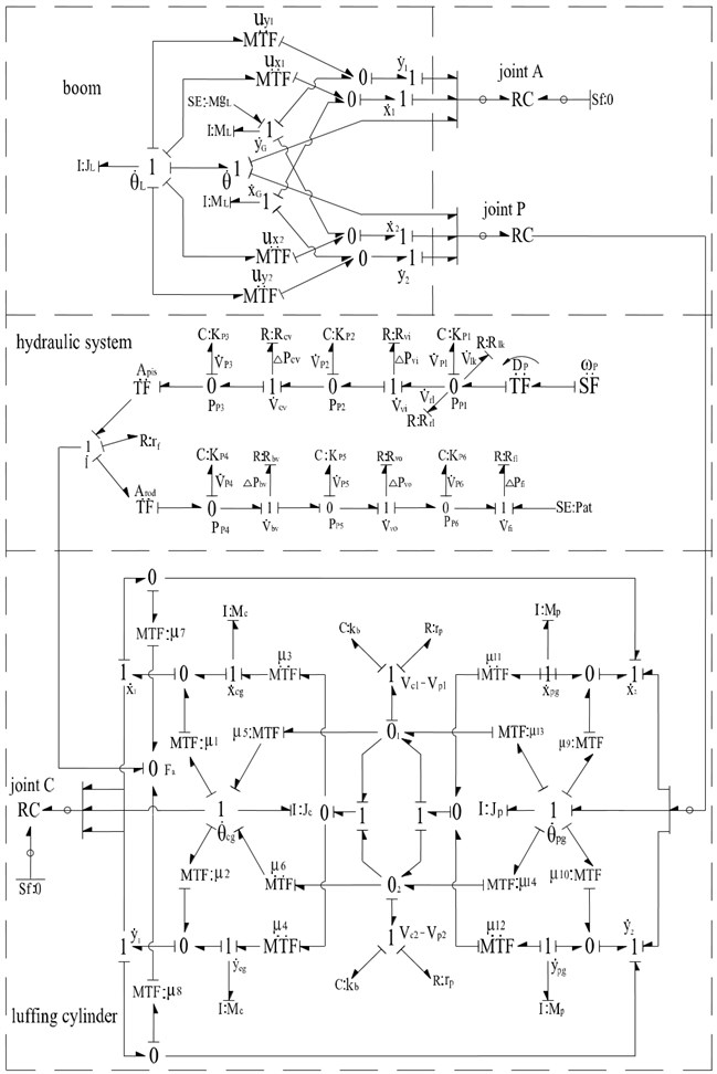
Fig. 11Experimental test set-up
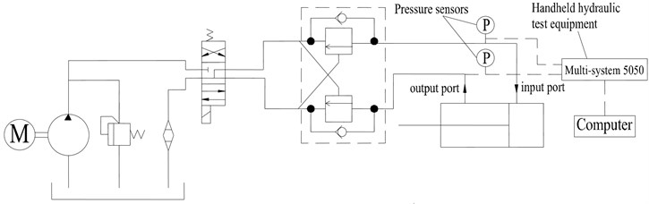
Fig. 12Photograph of the pressure sensors installation location of the luffing cylinder
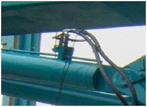
Table 1Main parameters for simulation
Parameter | Symbol | Value | Parameter | Symbol | Value |
The distance from point B to C / m | 1.05 | The distance from point C to P / m | 2.997 | ||
The distance from point A to P / m | 3.7 | The distance from point A to B / m | 1.4 | ||
The setting pressure of the unloading valve / MPa | 25 | The diameter of rod / m | 0.125 | ||
The speed of pump / r·min-1 | 1450 | The diameter of piston / m | 0.18 | ||
The displacement of pump / ml·r-1 | 107 | The mass of boom / Kg | 9.5×10³ | ||
Bulk modulus of the fluid / N·m5 | 7×10⁸ | The moment of inertial of boom / Kg·m2 | 2.74×10⁴ |
Fig. 13Comparison between experimental and simulation results of pressure in piston chamber
Fig. 14Comparison between experimental and simulation results of pressure in rod chamber
Fig. 13 and Fig. 14 show the comparison between the experimental data of chambers pressure of luffing cylinder and that of the simulation results. The follow conclusions can be made through analysis. (1) The actual completion time for luffing motion is 5 seconds longer than simulation results, and the experimental pressure curve has a degree of fluctuation. The reason is that the pulsation of the pump output flow is coupled with the vibration of the pipe, and the valve of the counterbalance valve is also vibrating during working process, what’s more, the leakage flow in the actual system is greater than that in simulation. (2) At the end of the luffing motion, the simulated pressure in the rod chamber is approximately 1.2 MPa higher than the measured value. This is due to the operation delay time of the directional control valve in actual system, while this isn’t taken into consideration in the simulation. This finding also means that reducing the closing time of the directional control valve will result in greater pressure shock. (3) After the completion of lifting the boom, the pressure in piston chamber is almost zero, and the pressure in rod chamber is stable at around 2 MPa. The final stable time is just 30 s in actual system, while it took about 65 s in simulation. The larger viscous damping coefficient in actual system may be the main reason for this difference. However, the close agreement between the two results and the similar pressure ripple characteristics can be seen in the two figures, which indicates that the model can be used to predict dynamic characteristics of the system.
6. Simulation results and discussion
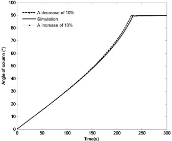
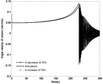
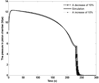
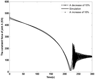
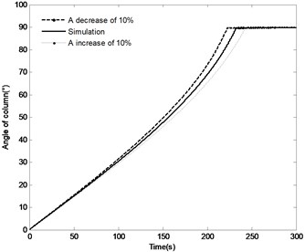
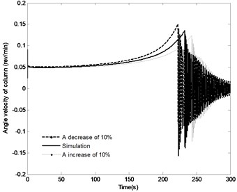
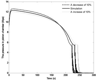
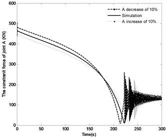
The effect of the change in the distance by the range of ±10 % on the angle of the boom, angle velocity of the boom, the pressure in the piston chamber and the constraint forces of joint A are shown in Fig. 15. The following conclusions can be made through analysis. With the distance increasing, the time to achieve the vertical position increases from 226.5 s to 239 s, while the angle velocity of boom decreases and the maximum pressure in the piston chamber decreases from 13 MPa to 11.8 MPa. It is also apparent that with the decrease in the distance , the initial constraint force of joint A increase from 424.5 KN to 597.5 KN. Specially, with full closing of the directional control valve, the fluctuation of the constraint force increase. However, the steady state constraint force is basically the same. It can be seen from the above results, change in the distance has great effect on the system response.
Fig. 15The effect of distance r4 on the system response
a) Angle of the boom
b) Angle velocity of the boom
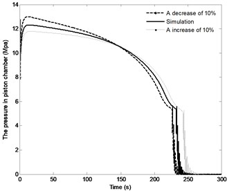
c) The pressure in piston chamber
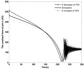
d) The constraint force of joint A
The effect of the change in the distance by the range of ±10 % on the angle of the boom, angle velocity of the boom, the pressure in the piston chamber and the constraint forces of joint A are shown in Fig. 16. With the distance increasing, the time to achieve the end position increases from 229 s to 235.5 s; the angle velocity of boom have small declines; the maximum pressure in the piston chamber is basically the same. It is also apparent that with the increase in the distance , the initial constraint force of joint A increases from 455.5 KN to 474.5 KN, when the directional control valve is fully closed, the fluctuation of the constraint force is also increased, however, the steady state of constraint force is basically the same. These finding indicate that change in the distance has little effects on the system responses. Therefore, this parameter is not a priority in the design phase.
Fig. 16The effect of distance r3 on the system response
a) Angle of the boom
b) Angle velocity of the boom
c) The pressure in piston chamber
d) The constraint force of joint A
Fig. 17The effect of distance r1 on the system response
a) Angle of the boom
b) Angle velocity of the boom
c) The pressure in piston chamber
d) The constraint force of joint A
The effect of the change in the distance by the range of ±10 % on the angle of the boom, angle velocity of the boom, the pressure in the piston chamber and the constraint forces of joint A are shown in Fig. 17. With the distance increasing, the time to achieve the vertical position increases from 222.5 s to 243 s, however, the angle velocity of boom as well as the fluctuation of velocity decreases, the maximum pressure in the piston chamber also decreases from 12.6 MPa to 12.1 MPa. It can also be found that with the increase in the distance , the initial constraint force of joint A decreases from 476.5 KN to 446.5 KN; at the complete closing of the directional valve, the fluctuation of this constraint force decrease, but the steady state value is basically the same. The above results confirm that change in the distance has most influence on the modeling results compared with the plots as shown in Fig. 15 and Fig. 16.
From these simulation studies, it can be concluded that the distance as well as are the important design variables for the response of the system. Reducing the value of distance and may increase the system response, however, it would be the cost of the increasing demand for the strength of component.
7. Conclusions
The inherent complex dynamic characteristics of luffing mechanism should be studied with one integrated model, so the complete bond graph of luffing system has been developed with the advantage of bond graph in modeling complex multi-energy domains system. The model can clearly reveal the transmission, transformation and consumption of the system energy, and predict system response that are difficult to measure experimentally, such as the constraint force of joint. Comparing the simulation results with experimental data indicates that the model fairly represents the dynamic behavior of the system.
The effects of variations in three installation position parameters include distance , and on dynamic characteristics of the system have been presented. It shows that and are more important than the other one parameter affecting the system performance. As result of decrement of and , the constraint forces of joint A and C increase. Therefore, the structure size is reduced with the cost of the increasing demand for the strength of component and the hydraulic system pressure.
It is further concluded that this work provides a good base for the design and optimization of the luffing mechanism. The dynamic analysis for the similar mechanism can also refer to this modeling method. In the next, more attention should paid on the closing time of directional valve to reduce the hydraulic shock, and the model can be refined by incorporating the dynamic behavior of the pump and hydraulic control valves.
References
-
Kang Hui-mei, He Qing-hua, Zhu Jian-xin. Dynamic modeling and simulation of mast link frame system of rotary drilling rig. Journal of Central South University, Science and Technology, Vol. 41, Issue 2, 2010, p. 532-538, (in Chinese).
-
Yang Hua Dynamic analysis on tunneling support system of the ZY-220 rotary drilling rig. Ph. D. Dissertation, Jilin University, 2007, (in Chinese).
-
Wang Peng-ju, Fang Yong-chun, Xiang Ji-lei, et al. Dynamics analysis and modeling of ship-mounted boom crane. Journal of Mechanical Engineering, Vol. 47, Issue 20, 2011, p. 34-40, (in Chinese).
-
Jiang Tao, You Yi-ping, Yang Hu, et al. Integrated model-based analysis of mast mechanism of rotary drilling rig and its dynamic characteristics. Journal of Tongji University, Vol. 40, Issue 5, 2012, p. 729-734, (in Chinese).
-
Xu Xue-song, Hu Ji-quan Hybrid neural networks based portal cranes’ luffing system optimal design. Chinese Journal of Mechanical Engineering, Vol. 41, Issue 4, 2005, p. 220-224, (in Chinese).
-
Lin Xiao-hui, Huang Wei, Lin Xiao-tong, et al. Study of synthetical genetics annealing optimization for the luffing mechanism locus of a plane link. Journal of Computer-Aided Design and Computer Graphics, Vol. 13, Issue 8, 2001, p. 724-729, (in Chinese).
-
Flores P. Modeling and simulation of wear in revolute clearance joints in multi-slewing platform systems. Mechanism and Machine Theory, Vol. 44, Issue 6, 2009, p. 1211-1222.
-
FilippovA. Vibrations of Mechanical systems. England, Yorkshire, Boston Spa, National Lending Library for Science and Technology, 1971.
-
Bera T. K., Samantaray A. K. Consistent bond graph modelling of planar multibody systems. World Journal of Modelling and Simulation, Vol. 7, Issue 3, 2011, p. 173-188.
-
Marquis-favre W., Bideaux E., Scavarda S. A planar mechanical library in the amesim simulation software. Part I: Formulation of dynamics equations. Simulation Modelling Practice and Theory, Vol. 14, Issue 1, 2006, p. 25-46.
-
Ahmed S., Lankarani H., Pereira M. Frictional impact analysis in open-loop multibody mechanical systems. Journal of Mechanical Design, Vol. 121, Issue 1, 1999, p. 119-127.
-
Karnopp D. C., Margolis D. L., Rosenberg R. C. System Dynamics: Modeling, Simulation, and Control of Mechatronic Systems. New York, John Wiley & Sons, 2012.
-
He Xiao-yan, Qin Si-cheng Finite element analysis for the triangular connecting frame of drill mast on rotary pile drill. Construction Machinery and Equipment, Vol. 38, Issue 10, 2007, p. 34-36, (in Chinese).
-
Zhu Jin-guang, Chen Min-ge, Liu An-ning, et al. Finite element analysis for the working equipment of drilling rigs. Agricultural Equipment & Vehicle Engineering, Issue 2, 2007, p. 24-27, (in Chinese).
-
Yi Wei, Zhou Hai-sheng, Zhao Li-ming, et al. Load analysis of hydraulic cylinder of lift-arm of rotary drilling rig. Annua1 Conference of China Pile Machinery Industry. Changsha, 2006, p. 31-33, (in Chinese).
-
Zhu Jian-xin, Xie Song-yue, Hu Xiong-wei, et al. Simulation analysis of the lifting force of parallelogram cylinder of the parallelogram system of rotary drilling rig based on ADAMS. Modern Manufacturing Engineering, Vol. 11, 2009, p. 119-123, (in Chinese).
-
Wang Zi-po, Hu Jun-ke, Yang Wen-bin, et al. Research on the stability of boom luffing mechanism at decline stage. Journal of Hefei University of Technology, Vol. 36, Issue 7, 2013, p. 783-787, (in Chinese).
-
Wang Tong-jian, Chen Jin-shi, Zhao Qing-bo, et al. Mechanical-hydraulic co-simulation and experiment of full hydraulic steering system. Journal of Jilin University: Engineering and Technology, Vol. 43, Issue 3, 2013, p. 607-612, (in Chinese).
About this article

