Design and simulation analysis of an improved lower limb exoskeleton

Li, Na; Yan, Lei; Qian, Hua; Wu, Jian; Men, Sen; Li, Yanbei

Journal of Vibroengineering

Browse Journal

Submit article

Published: 15 November 2014

Check for updates

Design and simulation analysis of an improved lower limb exoskeleton

Na Li¹

Lei Yan²

Hua Qian³

Jian Wu⁴

Sen Men⁵

Yanbei Li⁶

^{1, 2, 3, 4, 5, 6}School of Technology, Beijing Forestry University, Beijing, China

Corresponding Author:

Hua Qian

Cite the article Download PDF

Downloads 1635

Abstract

The lower extremity exoskeleton robot is a type of power assisted robot which can enhance the human walking function. A fundamental problem in the development of the exoskeleton is the choice of lightweight actuators. Thus in the mechanical structure design in this paper, the linear motor is selected as it greatly reduces the complexity of the mechanical structure. Furthermore, the limit switch inside the motor improves the safety performance. Based on the last version of the exoskeleton, the band positions, length adjusting holes and mechanical limit structures are increased. In addition, a control system based on DSP is designed. Furthermore, a kinematics analysis is carried out using the D-H parameter method and a dynamic analysis is developed using the Newton-Euler method. The driving force of every joint is obtained during the simulation using ADAMS software.

1. Introduction

Recently, lower limb exoskeletons have become a subject of great research interest as they run parallel to a wearer’s legs. Exoskeletons can perform particular functions such as: walking assistance; carrying a heavy burden; and physical therapy support for patients who are unable to walk again. However, portable power supplies, lightweight actuators and high-efficiency transmissions are some of the most important factors that still need to be improved [1].

A brief summary of the commercial exoskeleton is presented below.

Currently, about four kinds of exoskeletons are commercially available: HAL, ReWalk, eLEGS and Rex. The latest version of HAL has 3 active joints with 1 degree of freedom (DoF) at the hip, the knee and the ankle. Otherwise HAL is designed to only be worn on one side of the body. Rex provides an actuated flexion/extension of the hip, the knee and the ankle, as well as hip abduction/adduction and ankle inversion/eversion. It does not need additional support to maintain a balance, like crutches, but it is only used by patients who sit in wheelchairs and operate hand controls. ReWalk and eLEGS actively support the flexion/extension at the knee and the hip joints, and the wearers of both would need walking sticks to maintain a balance.

Other exoskeletons still remain at a research stage, for example SUBAR and WPAL.

An exoskeleton has been designed in the author’s laboratory to improve the walking ability of the elderly with linear actuators. Thus a simple and convenient actuation module makes an exoskeleton more compact. The first version of a lower limb exoskeleton has been designed, as shown in Fig. 1. However, in experiments some shortcomings limited the robot’s ability to work with humans. In this paper, the improved version is introduced. The structure of the paper is as follows: the mechanical design is demonstrated in Section 2; the kinematic and dynamic analyses are performed in Sections 3 and 4; and finally, conclusions are drawn in Section 5.

2. The hardware design of the lower limb exoskeleton

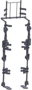
The exoskeleton is a type of robot which is integrated with the wearer’s body. An improved version is introduced in this section. The lower limb exoskeleton is designed with 2 active actuators at the hip and knee and the ankle has 1 DoF without an actuator. A design of the improved version can be seen in Fig. 2. A circular pipe shape has been selected for the thigh and shank because of its lightness and ease of processing. Aluminum is the main material used due to its lightness and inexpensiveness [2-6].

Fig. 1The first version of the lower limb exoskeleton

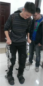
Fig. 2The improved version

2.1. The length adjustment in the thigh, shank and waist

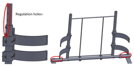
To make it comfortable for the wearer, an exoskeleton is supposed to be adjustable in length. The ratio of the body part to height, which ranges from 160 cm to 180 cm, is shown in Fig. 3. Thus the variation range is approximately 6 cm for the thigh and shank and 3 cm for the waist. The mechanical design is shown in Fig. 4. The length of the thigh and shank can be fixed at 390 mm, 410 mm, 430 mm or 450 mm, and the length of waist can be fixed at 392 mm, 408 mm or 424 mm. The regulation holes are circled in red.

Fig. 3The ratio of the body part to its height

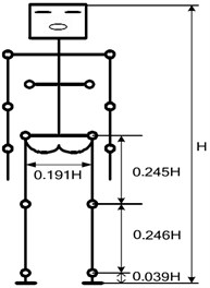
Fig. 4The mechanical design of the thigh, shank and waist

2.2. The stop block of the knee

Careful consideration should be given to safety issues when designing the exoskeleton, especially in the knee. In the sagittal plane, the rotation range of the knee is about –120 degrees to 0 degrees. To avoid the knee joint going beyond this range, a stop block module is installed at the knee. As shown in the Fig. 5, the module is painted green. When the red borders of the joint run into the stop block, the knee will rotate to the limit position. Because a human’s hip can extend or flex in a wide range, no limit block is installed in the hip joint.

2.3. The actuator

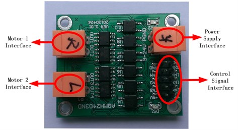
Electric motors have been selected for the actuator due to their convenience and compact structure, when compared to a hydraulic actuator. The linear motor, which has been remade as shown in Fig. 6, is chosen as the actuator due to its several advantages. First of all, its output is a linear motion and the mechanical structure design is greatly simplified. Moreover, the limit switches are installed on both ends of the range, which ensures the wearer’s safety. The stroke of the DC motor is 100 mm, it needs 24 V power supply and its normal rated thrust is 2000 N. When the positive and negative poles of input power are exchanged, the motor will change its direction of motion. The motor controller that is matched to the linear motor is adopted, as shown in Fig. 7. One motor controller can control two motors at the same time.

Fig. 5The stop block of the knee

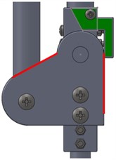
Fig. 6The linear motor

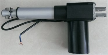
Fig. 7The motor controller

2.4. The control system design

Since multi-sensor data fusion has been selected as a control method for the synchronization of the robot and human body, the positions of the thigh and the shank that are detected by sensors should be known. Thus IMU sensors are attached to the thigh and shank to receive motion information and encoders are installed at each joint to measure the rotation. The linear displacement transducers are installed with the DC motors to check their distance range and force sensors are installed on the surface of the feet to detect the distribution of gravity.

There are 4 DSP modules for controlling the exoskeleton. One is the main module for calculating and saving data. Two DSPs are used to collect information from the sensors fixed on the left and right legs, which they then send to the main DSP by CAN (Controller Area Network). The main DSP then sends orders to the last DSP which controls the linear motors.

3. Kinematic analysis

Following the overview of the mechanical design, the motion process will be introduced in this section.

There are three rotary motions on each leg of the lower limb exoskeleton. The waist, thigh and shank are considered to be rigid links in the sagittal plane. Thus the exoskeleton consists of a series structure with six DoFs [9, 10].

Firstly, the standing posture is defined as the initial position. The origin $O$ of the base coordinate system $O X Y Z$ is selected at the right ankle. The $X$ axis is horizontally forward. Then the coordinate system $O_{1} X_{1} Y_{1} Z_{1}$ is established at the right ankle, and the origin $O_{1}$ coincides with the origin $O$ . The $Z$ axis is perpendicular to the surface, and coincides with the spin axis of the joint. The $X$ axis is along the direction of the shank, and the $Y$ axis is determined by the right-hand rules. The other coordinate systems are set up in the same way, as shown in Fig. 8. The D-H link parameters for the exoskeleton are shown in Table 1.

Fig. 8The D-H model of the exoskeleton and axes on the joints

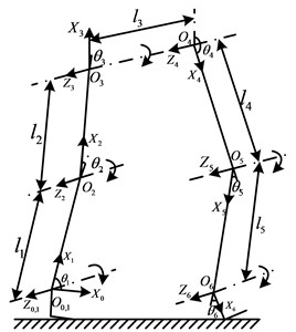
Table 1The D-H link parameters for the exoskeleton

$i$	$θ_{i}$	$α_{i}$	$a_{i}$	$d_{i}$
1	$θ_{1}$	0	0	0
2	$θ_{2}$	0	$l_{1}$	0
3	$θ_{3}$	0	$l_{2}$	0
4	$θ_{4}$	0	0	$l_{3}$
5	$θ_{5}$	0	$l_{4}$	0
6	$θ_{6}$	0	$l_{5}$	0

The link transformation matrix between the neighboring coordinate systems can be expressed by the generalized transformation matrix formula, as provided in Eq. (1):

1

A_{i} = R o t (z, θ_{i}) T r a n s (0,0, d_{i}) T r a n s (a_{i}, 0,0) R o t (x, α_{i}) .

Then the link transformation matrix $A_{1}$ between coordinate $O X Y Z$ and coordinate $O_{1} X_{1} Y_{1} Z_{1}$ can be expressed using the following Eq. (2):

2

A_{1} = R o t (z, θ_{1}) T r a n s (0,0, d_{1}) T r a n s (a_{1}, 0,0) R o t (x, α_{1})

= R o t (z, θ_{1}) T r a n s (0,0, 0) T r a n s (0,0, 0) R o t (x, 0)

= [\begin{matrix} c o s θ_{1} & - s i n θ_{1} & 0 & 0 \\ s i n θ_{1} & c o s θ_{1} & 0 & 0 \\ 0 & 0 & 1 & 0 \\ 0 & 0 & 0 & 1 \end{matrix}] [\begin{array}{l} 1 & 0 & 0 & 0 \\ 0 & 1 & 0 & 0 \\ 0 & 0 & 1 & 0 \\ 0 & 0 & 0 & 1 \end{array}] = [\begin{matrix} c o s θ_{1} & - s i n θ_{1} & 0 & 0 \\ s i n θ_{1} & c o s θ_{1} & 0 & 0 \\ 0 & 0 & 1 & 0 \\ 0 & 0 & 0 & 1 \end{matrix}] .

In the same way, when $i = 2, 3, 5, 6$ , the matrix $A_{i}$ from the $i -$ 1th to the $i$ th coordinate, may be constructed as:

3

A_{i} = R o t (z, θ_{i}) T r a n s (0,0, 0) T r a n s (l_{i - 1}, 0,0) R o t (x, 0)

= [\begin{matrix} c o s θ_{i} & - s i n θ_{i} & 0 & 0 \\ s i n θ_{i} & c o s θ_{i} & 0 & 0 \\ 0 & 0 & 1 & 0 \\ 0 & 0 & 0 & 1 \end{matrix}] [\begin{array}{l} 1 & 0 & 0 & l_{i - 1} \\ 0 & 1 & 0 & 0 \\ 0 & 0 & 1 & 0 \\ 0 & 0 & 0 & 1 \end{array}] = [\begin{matrix} c o s θ_{i} & - s i n θ_{i} & 0 & l_{i - 1} c o s θ_{i} \\ s i n θ_{i} & c o s θ_{i} & 0 & 0 \\ 0 & 0 & 1 & 0 \\ 0 & 0 & 0 & 1 \end{matrix}] .

Additionally matrix $A_{4}$ from coordinate $O_{3} X_{3} Y_{3} Z_{3}$ to $O_{4} X_{4} Y_{4} Z_{4}$ can be expressed as:

4

A_{4} = R o t (z, θ_{4}) T r a n s (0,0, l_{3}) T r a n s (0,0, 0) R o t (x, 0)

= [\begin{matrix} c o s θ_{4} & - s i n θ_{4} & 0 & 0 \\ s i n θ_{4} & c o s θ_{4} & 0 & 0 \\ 0 & 0 & 1 & 0 \\ 0 & 0 & 0 & 1 \end{matrix}] [\begin{array}{l} 1 & 0 & 0 & 0 \\ 0 & 1 & 0 & 0 \\ 0 & 0 & 1 & l_{3} \\ 0 & 0 & 0 & 1 \end{array}] = [\begin{matrix} c o s θ_{4} & - s i n θ_{4} & 0 & 0 \\ s i n θ_{4} & c o s θ_{4} & 0 & 0 \\ 0 & 0 & 1 & l_{3} \\ 0 & 0 & 0 & 1 \end{matrix}] .

Thus, the position and posture at the end of exoskeleton can be represented in the base coordinate system as:

5

A = A_{1} A_{2} A_{3} A_{4} A_{5} A_{6} = [\begin{array}{l} n_{x} & o_{x} & a_{x} & p_{x} \\ n_{y} & o_{y} & a_{y} & p_{y} \\ n_{z} & o_{z} & a_{z} & p_{z} \\ 0 & 0 & 0 & 1 \end{array}] .

The posture at the end in the base coordinate is:

6

R_{6} = [\begin{array}{l} n_{x} & o_{x} & a_{x} \\ n_{y} & o_{y} & a_{y} \\ n_{z} & o_{z} & a_{z} \end{array}] .

And the position at the end in the base coordinate is:

7

T_{6} = {[\begin{array}{l} p_{x} & p_{y} & p_{z} \end{array}]}^{T} .

In order to determine its precision, the special values when the exoskeleton is standing upright are taken into Eq. (5).

Where: $θ_{1} =$ 90°, $θ_{2} =$ 0°, $θ_{3} =$ 0°, $θ_{4} =$ 180°, $θ_{5} =$ 0°, $θ_{6} =$ 0°.

The matrix $A$ becomes Eq. (8), which is consistent with the actual situation:

8

A = [\begin{matrix} 0 & 1 & 0 & 0 \\ - 1 & 0 & 0 & 0 \\ 0 & 0 & 1 & l_{3} \\ 0 & 0 & 0 & 0 \end{matrix}] .

4. Dynamic analysis and simulation

The aim of this section is to test and verify whether the motor’s driving force is suitable. In order to do this the Newton-Euler method is adopted and a simulation is carried using the ADAMS software.

4.1. The Newton-Euler dynamic formulation

Using Fig. 8 as a basis, the Newton-Euler Dynamic Formulation is used to solve its dynamic equation.

Firstly, the rotation matrixes for each coordinate system are as follows:

9

{}^{i - 1} T_{i} = [\begin{matrix} c o s θ_{i} & - s i n θ_{i} & 0 \\ s i n θ_{i} & c o s θ_{i} & 0 \\ 0 & 0 & 1 \end{matrix}], {}^{i} T_{i - 1} = [\begin{matrix} c o s θ_{i} & s i n θ_{i} & 0 \\ - s i n θ_{i} & c o s θ_{i} & 0 \\ 0 & 0 & 1 \end{matrix}] .

Thus:

\begin{array}{l} {}^{0} T_{2} = {}^{0} T_{1} {}^{1} T_{2}, {}^{0} T_{3} = {}^{0} T_{2} {}^{2} T_{3}, {}^{0} T_{4} = {}^{0} T_{3} {}^{3} T_{4}, {}^{0} T_{5} = {}^{0} T_{4} {}^{4} T_{5}, {}^{0} T_{6} = {}^{0} T_{5} {}^{5} T_{6}, \\ {}^{2} T_{0} = {}^{2} T_{1} {}^{1} T_{0}, {}^{3} T_{0} = {}^{3} T_{2} {}^{2} T_{0}, {}^{4} T_{0} = {}^{4} T_{3} {}^{3} T_{0}, {}^{5} T_{0} = {}^{5} T_{4} {}^{4} T_{0}, {}^{6} T_{0} = {}^{6} T_{5} {}^{5} T_{0} . \end{array}

The initial conditions are listed as follows:

ω_{0} = {\dot{ω}}_{0} = υ_{0} = 0, {\dot{υ}}_{0} = {(\begin{array}{l} 0 & g & 0 \end{array})}^{T} .

4.1.1. The calculation of each joint’s angular velocity

The angular velocity of rotary joint 1 is:

10

{}^{1} T_{0} ω_{1} = {}^{1} T_{0} (ω_{0} + Z_{0} {\dot{θ}}_{1}),

where $Z_{0} = {[\begin{array}{l} 0 & 0 & 1 \end{array}]}^{T}$ .

In the same way, when $i = 2, 3, 4, 5, 6$ , the angular velocity of rotary joint $i$ is:

11

{}^{i} T_{0} ω_{i} = {}^{i} T_{i - 1} ({}^{i - 1} T_{0} ω_{i - 1} + Z_{0} {\dot{θ}}_{i}) .

4.1.2. The calculation of each joint’s angular acceleration

The angular acceleration of rotary joint 1 is:

12

{}^{1} T_{0} {\dot{ω}}_{1} = {}^{1} T_{0} ({\dot{ω}}_{0} + Z_{0} {\ddot{θ}}_{1} + ω_{0} \times Z_{0} {\dot{θ}}_{1}) .

In the same way, when $i = 2, 3, 4, 5, 6$ , the angular acceleration of rotary joint $i$ is:

13

{}^{i} T_{0} {\dot{ω}}_{i} = {}^{i} T_{i - 1} ({}^{i - 1} T_{0} {\dot{ω}}_{i - 1} + Z_{0} {\ddot{θ}}_{i} + ({}^{i - 1} T_{0} ω_{i - 1}) \times Z_{0} {\dot{θ}}_{i}) .

4.1.3. The calculation of each joint’s linear acceleration

The position vector of the origin $O_{i}$ in the coordinate system whose origin is $O_{i - 1}$ is $p_{i}^{*}$ .

The linear acceleration of rotary joint 1 is:

14

{}^{1} T_{0} {\dot{υ}}_{1} = ({}^{1} T_{0} {\dot{ω}}_{1}) \times ({}^{1} T_{0} p_{1}^{*}) + ({}^{1} T_{0} ω_{1}) \times [({}^{1} T_{0} ω_{1}) \times ({}^{1} T_{0} p_{1}^{*})] + {}^{1} T_{0} {\dot{υ}}_{0},

where $p_{1}^{*} = {[\begin{array}{l} 0 & 0 & 0 \end{array}]}^{T}$ .

In the same way, when $i = 2, 3, 4, 5, 6$ , the linear acceleration of rotary joint $i$ is:

15

{}^{i} T_{0} {\dot{υ}}_{i} = ({}^{i} T_{0} {\dot{ω}}_{i}) \times ({}^{i} T_{0} p_{i}^{*}) + ({}^{i} T_{0} ω_{i}) \times [({}^{i} T_{0} ω_{i}) \times ({}^{i} T_{0} p_{i}^{*})] + {}^{i} T_{i - 1} ({}^{i - 1} T_{0} {\dot{υ}}_{i - 1}),

where ${}^{i} T_{0} p_{i}^{*} = {[\begin{array}{l} l_{i - 1} & 0 & 0 \end{array}]}^{T}$ ( $i =$ 2, 3, 5, 6), ${}^{4} T_{0} p_{4}^{*} = {[\begin{array}{l} 0 & 0 & l_{3} \end{array}]}^{T} .$

4.1.4. The calculation of the centroid acceleration of each link

The origin of the base coordinate system and coordinate system $O_{1} X_{1} Y_{1} Z_{1}$ is the same. Therefore link 1 can be thought of as the place where the two endpoints coincide. The centroid acceleration of link 1 is equal to the linear acceleration of rotary joint 1 as expressed in Eq. (16):

16

{}^{1} T_{0} a_{1}^{c} = {}^{1} T_{0} {\dot{υ}}_{1} .

When $i = 2, 3, 4, 5, 6$ , the centroid acceleration of link $i$ is:

17

{}^{i} T_{0} a_{i}^{c} = ({}^{i} T_{0} {\dot{ω}}_{i}) \times ({}^{i} T_{0} s_{i}) + ({}^{i} T_{0} ω_{i}) \times [({}^{i} T_{0} ω_{i}) \times ({}^{i} T_{0} s_{i})] + {}^{i} T_{0} {\dot{υ}}_{i},

where ${}^{i} T_{0} s_{i} = (\begin{array}{l} - l_{i - 1} / 2 & 0 & 0 \end{array})^{T}$ ( $i =$ 2, 3, 5, 6), ${}^{4} T_{0} s_{4} = {[\begin{array}{l} 0 & 0 & - l_{3} / 2 \end{array}]}^{T} .$

4.1.5. The calculation of the force on each link

The force on link 6 is:

18

{}^{6} T_{0} f_{6} = m_{6} {}^{6} T_{0} a_{6}^{c} .

When $i = 1, 2, 3, 4, 5$ , the force on link $i$ is:

19

{}^{i} T_{0} f_{i} = {}^{i} T_{i + 1} ({}^{i + 1} T_{0} f_{i + 1}) + m_{i} {}^{i} T_{0} a_{i}^{c} .

4.1.6. The calculation of the torque on each link

The inertia matrix of link $i$ relative to its centroid in coordinate system $(X_{0}, Y_{0}, Z_{0})$ is $I_{i}$ .

The torque on link 6 is:

20

{}^{6} T_{0} n_{6} = ({}^{6} T_{0} p_{6}^{*} + {}^{6} T_{0} s_{6}) \times (m_{6} {}^{6} T_{0} a_{6}^{c}) + {}^{6} T_{0} N_{6},

where the total external torque on link 6 is:

21

{}^{6} T_{0} N_{6} = ({}^{6} T_{0} I_{6} {}^{0} T_{6}) ({}^{6} T_{0} {\dot{ω}}_{6}) + ({}^{6} T_{0} ω_{6}) \times [({}^{6} T_{0} I_{6} {}^{0} T_{6}) ({}^{6} T_{0} ω_{6})] .

When $i = 1, 2, 3, 4, 5$ , the torque on link $i$ is:

22

{}^{i} T_{0} n_{i} = {}^{i} T_{i + 1} [{}^{i + 1} T_{0} n_{i + 1} + ({}^{i + 1} T_{0} p_{i}^{*}) \times ({}^{i + 1} T_{0} f_{i + 1})]

+ ({}^{i} T_{0} p_{i}^{*} + {}^{i + 1} T_{0} s_{i}) \times (m_{i} {}^{i} T_{0} a_{i}^{c}) + {}^{i} T_{0} N_{i} .

The total external torque on link $i$ is:

23

{}^{i} T_{0} N_{i} = ({}^{i} T_{0} I_{i} {}^{0} T_{i}) ({}^{i} T_{0} {\dot{ω}}_{i}) + ({}^{i} T_{0} ω_{i}) \times [({}^{i} T_{0} I_{i} {}^{0} T_{i}) ({}^{i} T_{0} ω_{i})] .

4.1.7. The calculation of the torque on each joint’s actuator

The torque of the actuator on joint 6 is:

24

τ_{6} = {({}^{6} T_{0} n_{6})}^{T} ({}^{6} T_{5} Z_{0}) .

When $i = 1, 2, 3, 4, 5$ , the torque of the actuator on joint $i$ is:

25

τ_{i} = {({}^{i} T_{0} n_{i})}^{T} ({}^{i} T_{i - 1} Z_{0}) .

4.2. Dynamics simulation

For the purposes of the simulation the three-dimensional model made by SolidWorks is imported into the ADAMS software [11]. The exoskeleton is then divided into seven parts and each part is dyed a different color, as shown in Fig. 9. There are two masses on the exoskeleton’s feet that imitate a human’s legs. The driving function on each joint is set according to the motion data of the human lower extremity joint.

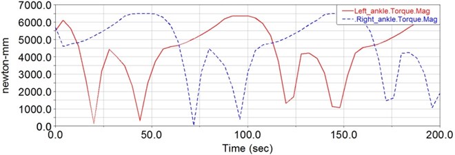
Following the simulation, the driving force of each joint can be obtained from the ADAMS/Postprocessor module. As shown in Fig. 10, this is the variation curve of the hip joint’s driving force. Whereas, in Fig. 11, it is the variation curve of knee joint’s driving force. The variation curve of the ankle joint’s driving torque is shown in Fig. 12. Thus the biggest driving force of the hip joint is about 2000 N, the biggest driving force of the knee joint is about 600 N and the biggest driving torque of the ankle joint is about 6.5 Nm. Because the driving torque of the ankle joint is far less than that of the knee and the hip joint, there is no actuator on the ankle joint. Therefore, it can be seen that the linear motors are appropriate for the improved design in this paper.

Fig. 9The simulation

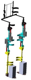
Fig. 10The required driving force of the hip joint

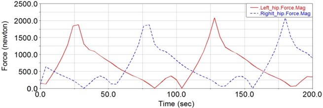
Fig. 11The required driving force of the knee joint

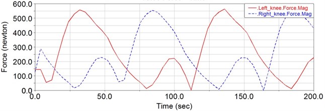
Fig. 12The required driving torque of the ankle joint

5. Conclusions

In this paper, a type of lower limb power assisted exoskeleton for the elderly has been designed. Based on human-machine coordination, the mechanical structure was improved by increasing the band positions, stop blocks and other factors. The control system which is based on DSP and multi-sensors has been introduced and kinematics analysis has been carried out according to the D-H parameter method. Furthermore, the parameters of the special positions were brought into equations to verify the imprecision, and these were seen to be consistent with the actual situation. The dynamics modeling analysis of the exoskeleton was developed by using the Newton Euler method and subsequently the required driving force of each joint of the lower extremity was obtained. Using ADAMS software, the 3D model was simulated as if it was a real situation. Subsequently the driving force of the hip, knee and ankle joint were attained, which provided an important reference for the selection of the motor. The dynamics analysis in this paper provided an important foundation for the control system and also offered a significant reference for the study of a humanoid robot’s dynamic walking.

References

Viteckova S., Kutilek P., Jirina M. Wearable lower limb robotics: A review. Biocybernetics and Biomedical Engineering, Vol. 33, Issue 2, 2013 p. 96-105.

Search CrossRef
Kim J. H., Han J. W., Kim D. Y., et al. Design of a walking assistance lower limb exoskeleton for paraplegic patients and hardware validation using CoP. International Journal of Advanced Robotic Systems, Vol. 10, 2013.

Search CrossRef
Yu H., Cruz M. S. T. A., Chen G., et al. Mechanical design of a portable knee-ankle-foot robot. IEEE International Conference on Robotics and Automation (ICRA), 2013, p. 2183-2188.

Search CrossRef
Costa N., Caldwell D. G. Control of a biomimetic soft-actuated 10 DOF lower body exoskeleton. The First IEEE/RAS-EMBS International Conference on Biomedical Robotics and Biomechatronics, 2006, p. 495-501.

Search CrossRef
Onen U., Botsali F. M., Kalyoncu M., et al. Design and actuator selection of a lower extremity exoskeleton. IEEE/ASME Transactions on Mechatronics, Vol. 19, Issue 2, 2013, p. 623-632.

Search CrossRef
Raj A. K., Neuhaus P. D., Moucheboeuf A. M., et al. Mina: a sensorimotor robotic orthosis for mobility assistance. Journal of Robotics, Vol. 2011, 2011.

Search CrossRef
Narong Aphiratsakun, Kittipat Chairungsarpsook, Manukid Parnichkun ZMP based gait generation of AIT’s leg exoskeleton. The 2nd International Conference on Computer and Automation Engineering (ICCAE), Vol. 5, 2010, p. 886-890.

Search CrossRef
Aaron M. Dollar, Aaron M. Dollar Lower extremity exoskeletons and active orthoses: Challenges and state-of-the-art. IEEE Transactions on Robotics, Vol. 24, Issue 1, 2008, p. 1-15.

Search CrossRef
Miao Y., Gao F., Pan D. State classification and motion description for the lower extremity exoskeleton SJTU-EX. Journal of Bionic Engineering, Vol. 11, Issue 2, 2014, p. 249-258.

Search CrossRef
Bing Lei Structure Optimization and Performance Evaluation of Leg Exoskeleton for Load-Carrying Augment. East China University of Science and Technology, 2011.

Search CrossRef
Yali Han, Xingsong Wang Dynamic analysis and simulation of lower limb power-assisted exoskeleton. Journal of System Simulation, Vol. 25, Issue 1, 2013.

Search CrossRef
Anam K., Al-Jumaily A. A. Active exoskeleton control systems: state of the art. Procedia Engineering, Vol. 41, 2012, p. 988-994.

Search CrossRef
Jiafan Zhang, Ying Chen, Canjun Yang Human Intelligence System and Flexible Exoskeleton. Science Press, 2011.

Search CrossRef
Jimenez-Fabian R., Verlinden O. Review of control algorithms for robotic ankle systems in lower-limb orthoses, prostheses, and exoskeletons. Medical Engineering and Physics, Vol. 34, Issue 4, 2012, p. 397-408.

Search CrossRef
Šlajpah S., Kamnik R., Munih M. Kinematics based sensory fusion for wearable motion assessment in human walking. Computer Methods and Programs in Biomedicine, Vol. 116, Issue 2, 2014, p. 131-144.

Search CrossRef
Vanderborght B., Albu-Schaeffer A., Bicchi A., et al. Variable impedance actuators: A review. Robotics and Autonomous Systems, Vol. 61, Issue 12, 2013, p. 1601-1614.

Search CrossRef
Hussain S., Xie S. Q., Jamwal P. K. Control of a robotic orthosis for gait rehabilitation. Robotics and Autonomous Systems, Vol. 61, Issue 9, 2013, p. 911-919.

Search CrossRef

About this article

Received

12 August 2014

Accepted

08 November 2014

Published

15 November 2014

Keywords

exoskeleton

kinematic analysis

simulation

Newton-Euler

Acknowledgements

This research was financially supported by the Fundamental Research Funds for the Central Universities (TD2013-3), China Postdoctoral Science Foundation (2013T60070) and Beijing Higher Education Young Elite Teacher Project (YETP0759).

This is an open access article distributed under the Creative Commons Attribution License, which permits unrestricted use, distribution, and reproduction in any medium, provided the original work is properly cited.