Analysis on aerodynamic characteristics and noise of the high-speed train under high-speed operation

2.1. Mathematical model for calculating the flow field of the high-speed train

For an operation train, its external flow field can be approximated as an incompressible viscous flow field, and the basic control equation is shown as follows:

where $u_i$, $u_j$ are the air velocity components in the flow field around the train. $x_i$, $x_j$ are the rectangular coordinate components. $\rho$ is the air density of the flow field around the train. $p$ is the air pressure of the flow field around the train. $\mu$ indicates the aerodynamic viscosity. $t$ is time.

A Realizable $k$-$\epsilon$ turbulence model was used to calculate the steady-state flow field. The model was proposed by Shih [9], and it is widely used to calculate flow field such as homogeneous shear flow field, boundary layer flow field and cavity flow field.

Transport equations of the Realizable $k$-$\epsilon$ turbulence model about $k$ and $\epsilon$ are as follows:

where, $G_k$ and $G_b$ are respectively generation items of turbulence energy $k$ caused by average velocity gradient and buoyancy. $Y_M$ refers to contribution made by pulsation expansion. $C_{i\epsilon }$$(i=\text{1,}\text{2,}\text{3})$ is an empirical constant. ${\sigma }_k$ and ${\sigma }_{\epsilon }$ are respectively Prandtl values corresponding to turbulence energy and dissipation rate. $S_k$ and $S_{\epsilon }$ are source items defined by the user. $C_1$ and $A_0$ are empirical constants, wherein $C_1=\mathrm{m}\mathrm{a}\mathrm{x}(0.43,\eta /\eta +5)$, $A_0=4.0$. ${\mu }_t$ is viscosity coefficient of the turbulence flow, wherein ${\mu }_t=C_{\mu }(\rho k^2/\epsilon )$. $C_{\mu }$ is a variable, $C_{\mu }=1/(A_0+A_s{U}^{\mathrm{*}}k/\epsilon )$, wherein the detailed expressions and derivation processes of $A_s$ and $U^{\mathrm{*}}$ are shown in reference [9]. Approximate solution of $A_s$ is $A_{\mathrm{s}}=\sqrt{6}\mathrm{c}\mathrm{o}\mathrm{s}\left[1/3\mathrm{c}\mathrm{o}{\mathrm{s}}^{-1}\right(\sqrt{6}W\left)\right]$, $W=E_{ij}{E}_{jk}{E}_{ki}/(S_{ij}{S}_{ij}{)}^{1/2}$, $W$ is the average rotation strain rate, and$S$is the average strain. $U^{*}=\sqrt{S_{ij}{S}_{ij}+{\tilde{\mathrm{\Omega }}}_{ij}{\tilde{\mathrm{\Omega }}}_{ij}}$, ${\tilde{\mathrm{\Omega }}}_{ij}={\mathrm{\Omega }}_{ij}-2{\epsilon }_{ijk}{\omega }_k$ and ${\mathrm{\Omega }}_{ij}={\stackrel{-}{\mathrm{\Omega }}}_{ij}-{\epsilon }_{ijk}{\omega }_k$.

Compared with the standard $k$-$\epsilon$ model, two differences are mainly shown in the Realizable $k$-$\epsilon$ turbulence model. Firstly, a formula is added in terms of turbulence viscosity. Secondly, a new equation of dissipation rate is added. This equation is derived on the basis of the fluctuation equation of laminar flow velocity. In the formula, $c_{\mu }$ is no longer a constant, and the contents about curvature and rotation are introduced, so as to make it meet the constraint conditions for Reynolds stress. Due to these characteristics, results of Realizable $k$-$\epsilon$ turbulence model are made more consistent with the actual conditions in calculating pressure gradient boundary layer, rotational flow and flow separation. Currently, in numerical calculation for the external flow field of train, the calculation accuracy of Realizable $k$-$\epsilon$ turbulence model were applied and verified [10, 11].

For selecting wall function, the Reynolds number of the near wall area on the rigid train body surface is low when the train is operating. As a result, the development of turbulence is insufficient. Its fluctuation influence is not as large as molecular viscosity $k$-$\epsilon$ turbulence model is built for flows which turbulence develops sufficiently, and it is applicable to high Reynolds number. Therefore, wall function of semi-empirical formula should be adopted at near wall area. In other words, variables to be solved at the core area of the turbulence are associated to the physical quantities on the wall:

In the equation, $u^{+}$ is a non-dimensional velocity, $u^{+}=u/v^{\mathrm{*}}$. $v^{\mathrm{*}}$ is shear stress velocity. $\mathrm{\Gamma }$ is blending function, $\mathrm{\Gamma }=-a({\mathrm{y}}^{+}{)}^4/(1+b{y}^{+})$. $y^{+}$ is non-dimensional distance, $a=$ 0.01 and $b=$ 5.

2.2. Algorithm for calculating source of aerodynamic noise for the high-speed train

In many actual applications considering turbulence, continuous distribution in a broadband range is presented for the noise energy, which involves in broadband noise. Few calculation resource is consumed by the broadband acoustic source model. The strength of the noise source on the solid surface wall of the flow field can be quickly analyzed and preliminarily predicted by it. Under broadband noise source model, the noise energy generated in the entire flow field can be defined by quantizing the local contribution, and the noise source can be analyzed and extracted. In this way, the main factors for noise generation can be known. The currently common Proudman model was selected.

The generated acoustic energy by the isotropic turbulence is as follows:

For $k$ and $\epsilon$, the mentioned formula can be written as:

The sound power level is as Eq. (8):

where, $u$ is turbulence velocity. $l$ is characteristic length. $a_0$ is sound velocity. $\alpha$ is model constant. $M_t=\sqrt{2k}/a_0$.

According to the mentioned theory analysis, problem of the flow field noise can be predicted by the Proudman noise energy approximation formula based on the premise of high Reynolds number and low Mach number. The flow of the train during steady operation basically meets the requirement.

3.1. Model simplification

Limited by computer hardware, the real movement condition of the train cannot be completely simulated by the calculation model. Therefore, the calculation model needs to be simplified. The model is subject to the followed simplifications during building.

1) Three trains were simulated in this paper. In other words, the entire model consisted of a head train, a middle train and a tail train. The head train and the tail train had identical appearance.

2) Pantograph, bogie, wheels and the small devices under the train were removed. Meanwhile, according to the symmetry, half of the model was cut along the longitudinal symmetrical plane of the train body to save computer resource.

3) Operation condition was uniform linear motion without considering wind. Operation velocity was approximate 250 km/h.

4) Compressibility of air was ignored. The air could be considered as incompressible viscous fluid when the Mach number was less than 0.3, and such condition had a little error.

5) A cross-section of common single track railway was used as the tunnel, as shown in Fig. 1.

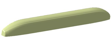
The simplification result of its profile was as shown in Fig. 2.

Fig. 1Cross-section of the tunnel for common single track railway

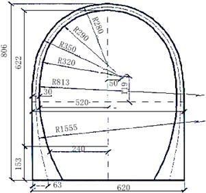
Fig. 2The geometrical model of a train

3.2. Boundary conditions, mesh generation and calculation

3.2.1. High-speed steady-state condition

The simplified three-dimensional model was imported into Gambit and T-Grid to generate mesh. A calculation domain with the length of 300 m, width of 11.5 m and height of 18 m was built. The entire calculation domain was divided into four parts by structured mesh. Such method was conducive to improving the calculation accuracy. Number of the mesh was 300,000. Then, boundary definition was carried out, and the front and back boundary was pressure-far-field. The bottom boundary was move-wall, and the upper and bottom surfaces of the train body model were walls. They were used for subsequent calculation and description of air flow field characteristics. The calculation mesh is as shown in Fig. 3 and Fig. 4.

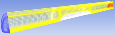
Fig. 3Planning of the flow field calculation domain outside the train

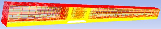
Fig. 4Mesh of the flow field near the train body

During calculation of the steady-state flow, the turbulence model used Realizable $k$-$\epsilon$ model. Some history effect was included in the turbulence viscosity coefficient of this model[12]. Turbulence viscosity coefficient as well as turbulent kinetic energy and its dissipation rate could be associated by it. Hence, the calculation accuracy of numerical simulation could be improved significantly. The enhanced wall function was taken as near wall function, and separation solver was taken as the solver. Compressible flow analysis was built by double precision solving, second order upwind scheme. SIMPLEC algorithm was adopted in the coupling calculation of pressure and velocity. In this way, the convergence solutions such as $p$, $u$, $v$ etc. of the flow field parameters could be acquired through iteration. Hence, a high calculation accuracy and stability could be obtained.

3.2.2. Train-tunnel coupling condition

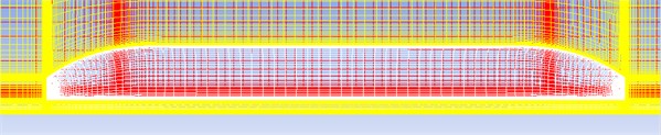
The domain of tunnel-train flow field was 100 m long. The entrance of flow field was 26 m away from the head of the train. The train body surface and the tunnel surface were triangle mesh. The calculation domain was tetrahedral mesh. The number of space volume mesh elements was 1.2 million as shown in Fig. 5. The front and back boundary was pressure-far-field, and the tunnel boundary was move-wall. The upper and bottom surfaces of the train body model were walls. They were used for subsequent calculation and description for air flow field characteristics.

Fig. 5Flow field mesh of tunnel-train

4.1. Analysis on the results of the external flow field for the train under steady-state

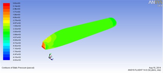
Air resistance of the train was 0.131, and aerodynamic lift was 0.98. The air moment against the head was –0.466. Meanwhile, according to Fig. 6-Fig. 9, when the train was under high-speed steady-state operation, the head was facing the stream. The air flow was prevented at the arc top. Hence, the velocity decreased significantly, almost reaching 0, as shown in Fig. 8.

Fig. 6Distribution of the pressure on the surface of the train

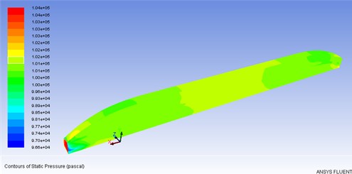
Fig. 7Distribution of the pressure in the external flow field of the train

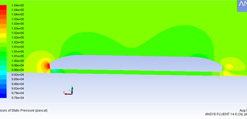
Fig. 8Velocity vector of the external flow field for the train

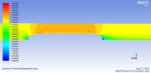
The flow field at the head was in positive pressure status. Meanwhile, the velocity of the external flow field reached the first negative pressure peak at the maximum cross-section of the train. Some air flow moved backward along both sides of the train and the upper curved surface. The flow velocity was accelerated by the change of curvature from the head to the train body. The positive pressure gradually decreased until it became negative pressure. The negative pressure reached maximum value at the head and the side surface. The second velocity peak occurred at the tail of the train, which was generated due to the acceleration of air flow velocity and the influence of the flow. The maximum velocity of flow field outside the train body reached 72.7 m/s. According to Fig. 10, when the maximum velocity was 4.7 m/s $<$ 14 m/s, passengers could bear at the position which was 2 m away from the train body. Such condition met the requirements of safe for human body.

Fig. 9Velocity curve of the flow field at the tail of the train

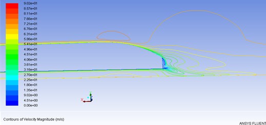
Fig. 10Velocity characteristics of the side for the train body

4.2. Analysis on the external flow field of the train under train-tunnel coupling

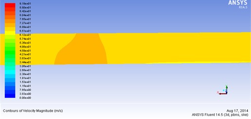
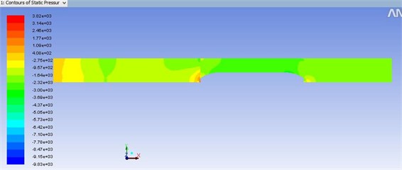
Air resistance of the train was 0.165, which was larger than the air resistance of steady-state condition, and aerodynamic lift was 3.75. Air moment against the head was –1.87. According to Fig. 11-Fig. 13, the tunnel wall near the head was positive pressure area. At this position, the value reached maximum peak. The pressure on the tunnel wall opposite to the train body distributed uniformly, and it was negative pressure area. Due to the prevention of the head, the air flow velocity decreased significantly, almost reaching 0 when the air flow passed the surface of the train.

Fig. 11Distribution of the pressure on the train surface in tunnel environment

Comparison with the aerodynamic characteristics in steady-state condition in Section 4.1.1 showed that the train suffered from larger resistance in tunnel environment than steady-state condition. The exceeded resistance was the additional air resistance in the tunnel. The resistance was caused by the pressure difference between the positive pressure at the head and the negative pressure at the tail. It was because the air was driven by the train when it entered into the tunnel. Hence, resistance was generated. Meanwhile, because of the train structure, turbulence flow will be caused by the air in the tunnel. Friction between the air and the train surface as well as the tunnel surface will be caused by the flow. Therefore, resistance resisting the train’s motion will be generated. The longer the tunnel is, the larger the resistance will be. The longer the train is, the larger the velocity will be, and the resistance will increase accordingly. In addition, this resistance is also related to the sectional area of the tunnel, train appearance etc.

Fig. 12Distribution and curve of the flow field velocity in the tunnel

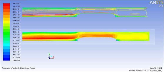
Fig. 13Distribution of the pressure of the external flow field for the train in the tunnel

5.1. Experimental research of aerodynamic noise

PULSE analyzer of B&K Company was used as test equipment in aerodynamic noise experiment of the high-speed train. During the test of the external sound pressure for a high-speed train under high-speed operation condition, a traditional microphone could not be used to obtain the accurate experimental results. Hence, an aviation microphone was installed on the outer surface of the train window to test the external sound pressure, as shown in Fig. 14. In this way, the accurate experimental results could be obtained under high-speed operation. Test process of the external sound pressure was shown in Fig. 15. A multi-channel signal collection equipment was used to obtain signals of microphone. Then, the obtained data signals were imported into a PULSE analyzer for processing. Sound pressure levels of train body surface under steady-state operation and tunnel-train coupling conditions were tested, respectively, as shown in Fig. 16 and Fig. 17.

It is shown in Fig. 16 and Fig. 17 that sound pressure of train body surface under the tunnel-train coupling condition exceeded that under the steady-state operation condition within the whole frequency range. It was mainly because that strong coupling was generated between train and tunnel during train operation. As a result, sound pressure of train body surface was strengthened.

Fig. 14Installation diagram of the high-speed train microphone

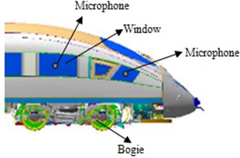
Fig. 15Test process of the external sound pressure for the high-speed train

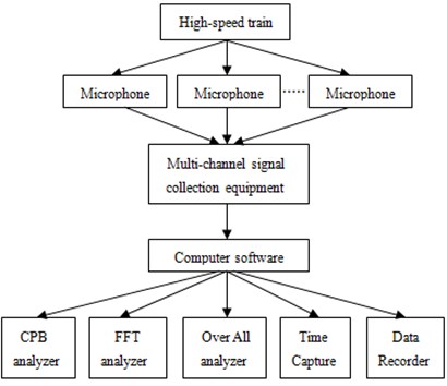
Fig. 16Sound pressure level of train body surface under steady-state operation condition

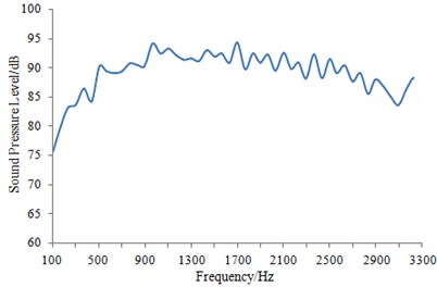
Fig. 17Sound pressure level of train body surface under tunnel-train coupling condition

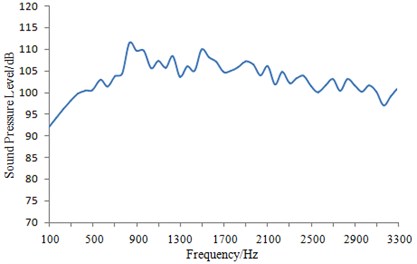
Fig. 18Relationship between sound pressure of train body surface and time when it went through a tunnel

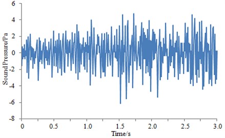
Signals which were obtained by the multi-channel data collection equipment were imported into Sound Quality software. And then, a curve for sound pressure of train body surface with time when a high-speed train entered into a tunnel under the operation speed of 250 km/h, as shown in Fig. 18. It is shown in the figure that fluctuation amplitude of the sound pressure curve suddenly increased at the time point of 1.5 s. On the one hand, air flow sound sharply increased at the instant when the train entered into the tunnel. On the other hand, the tunnel is equivalent to space with two opened ends while its inner wall surfaces are made of hard materials with very high reflection coefficients. As a result, the noise was much higher than that outside the tunnel. Such conclusion is consistent with the mentioned analysis results.

5.2. Numerical calculation of aerodynamic noise

Based on flow field of train body surface under steady-state operation condition, all parameters were consistent with experimental results, and then, numerical calculation was conducted to obtain sound power level of train body surface under the condition, as shown in Fig. 19.

Fig. 19Distribution of sound power level of the train body under steady-state operation condition

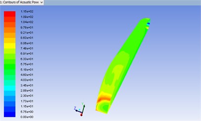
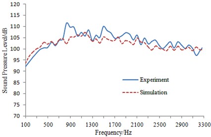
Fig. 20Experimental and simulated comparison of sound pressure level of train body surface under steady-state operation condition

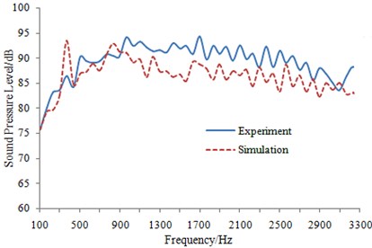
Sound power of train window in Fig. 19 was extracted, and it was transformed into sound pressure level and compared with experimental results in Fig. 16, as shown in Fig. 20.

It is shown in Fig. 20 that great differences were not shown by experimental results and simulated results in the whole analysis frequency range. In addition, the variation trends of experimental and simulated curves were consistent. Hence, the simulation model was deemed to be reliable, and it can be used to effectively predict aerodynamic noise of the high-speed train under steady-state operation.

According to Fig. 19, air flow speed increased due to the change of curved surface at the head. Because of the interaction between the boundary layer of the train body surface and the external flow field, the noise was high. Therefore, optimizing the shape of the head part for the train is an effective method to reduce the aerodynamic noise.

Sound power distribution of train body surface under the tunnel-train coupling state was obtained as shown in Fig. 21.

According to the method for obtaining sound power levels of train body surface under the steady-state operation condition. Sound powers at train window in Fig. 21 were extracted, and it was transformed into sound pressure levels and compared with experimental results in Fig. 17, as shown in Fig. 22.

It is shown in Fig. 22 that experimental results were relatively bigger than simulated results at frequencies of 900 Hz and 1500 Hz. It was because that certain error might be included in experimental results during test under so complicated environment. However, great differences were not shown in experimental and simulated results for the most frequencies within the whole frequency range. Moreover, the variation trends of both of them were basically consistent. Hence, the simulation model was deemed to be reliable, and it can be used to predict aerodynamic noise under tunnel-train coupling condition.

Fig. 21Distribution of sound power level of the train body under tunnel-train coupling condition

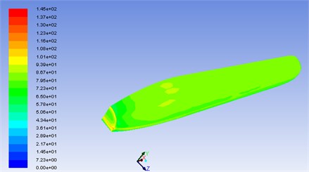
Fig. 22Experimental and simulated comparison of sound pressure level of train body surface under tunnel-train coupling condition

It is shown in Fig. 21 that sound power distribution of train body surface under this condition was basically consistent with that under steady-state condition. Hence, aerodynamic noise can be reduced by optimizing the train head.