Wind effects on a long span steel roof structure: numerical simulation and equivalent static wind loads

Fu, JiYang; Gao, Yun; Wu, JiuRong; Xu, An

Journal of Vibroengineering

Browse Journal

Submit article

Published: 15 August 2015

Check for updates

Wind effects on a long span steel roof structure: numerical simulation and equivalent static wind loads

JiYang Fu¹

Yun Gao²

JiuRong Wu³

An Xu⁴

^{1, 2, 3, 4}Tamkang University Joint Research Center for Engineering Structure Disaster Prevention and Control, Guangzhou University, Guangzhou 510006, China

Corresponding Author:

JiuRong Wu

Cite the article Download PDF

Downloads 1513

Abstract

A wind tunnel test is conducted in this study on the scaled model of the Guangzhou International Sports Arena (GISA). Simultaneous pressure measurements are conducted in a simulated suburban boundary layer flow field. A numerical simulation approach using Fuzzy Neural Networks (FNNs) is developed for the predictions of wind-induced pressure time series at roof locations which are not covered in the wind tunnel measurements. On the other hand, the wind-induced response of the roof are presented and discussed, which are directly calculated by the Complete Quadratic Combination (CQC) approach. Furthermore, the correlations between the background and resonant response components are discussed in detail, and the results show that neglecting the correlations between the two components would result in considerable error in the response estimation. Finally, the Equivalent Static Wind Load (ESWL) approach is used to estimate the wind-induced responses of the roof, which are compared with those obtained from the CQC approach to examine the effectiveness of the proposed ESWL approach in the design and analysis of large-span roof structures. It is shown through the example that the FNN and ESWL approaches can successfully predict the wind-induced pressures and responses respectively.

1. Introduction

In recent years, more and more large-span roof structures have been built or are being planned with increasing span and structural refinement throughout the world. Such roof structures usually have the characteristics of light mass, high flexibility, slight damping and low natural frequency. Consequently, these structures have become progressively more wind sensitive than most conventional roof structures, and wind loads generally control the design of these structures. In designing such large-span roof structures, it is usually necessary to conduct wind tunnel tests to determine wind loads on rigid models by taking pressure measurements. In these wind tunnel experiments, it needs to install as more pressure taps as possible on model surfaces in order to capture the detailed characteristics of wind loads on the structures; since variations of wind-induced pressures at different locations on surfaces of a roof are quite large [1]. Recent technological advances have made it possible to simultaneously measure surface pressures at more than 1000 locations on a building model [2], but such experimental arrangements may still not be able to cover the whole surfaces of a large-span roof structure. According to the requirement of wind tunnel tests, the density of arrangement in the pressure taps for long roof structures in the model test should be measured at a sufficient number of locations so that no significant aerodynamic events are missed. For a long span roof structure this may involve measurements at some 300 to 1000 or more locations, depending on the complexity of the exterior geometry. Some limitations exist for the High-Frequency Pressure-Integration (HFPI) method in the wind tunnel test. As for buildings with very complex shapes, or with many fine-scale features, such as long span roof with complex geometry, it is not possible to install enough pressure taps in all the required locations to accurately resolve the overall forces on the building. Until further experience is accumulated, the requisite number of simultaneously measured pressure taps ought to be judged with particular care and on a case by case basis.

Meanwhile a finite element model is often utilized for the numerical analysis of wind-induced response of large span roof structure. Normally the number of element nodes in finite element model is very large than the number of pressure taps arranged in the wind tunnel test. In order to obtain the information of aerodynamic wind load for unresolved element nodes in finite element model, the numerical interpolation or extrapolation methods is normally adopted. However the approximation accuracy for the kind of method could not be guaranteed as the physical phenomena of wind load distribution could difficultly obtained by the simple numerical interpolation or extrapolation method. Based on the above two mentioned requirements in wind tunnel test and/or wind-induced response analysis, there is a need to explore an effective approach for the prediction the wind-induced pressures which were not covered in the wind tunnel measurements and/or finite element model. Thus the wind-induced pressures on an entire large-span roof structure could be obtained from the pressure measurements with limited number of pressure taps in the wind tunnel test.

There are several useful ways to predict or simulate time series of random data such as wind-induced pressure. Among them there are the autoregressive moving average (ARMA) method [38, 39], the Fourier transform methods [40], and the wavelet transform method [41, 42], etc. The ARMA method has been well developed and successfully used for generation of wind-speed time series [38, 39]. However, the model was found to be inappropriate for generating time series of random data with non-Gaussian features. Another standard approach, the Fourier transform method [40], shows good performance for autocorrelation and power spectrum simulation, but it is also limited to the case of a Gaussian probability distribution. The wavelet transform method can capture the non-Gaussian and non-stationary features of time series of random data and it has been used for simulating the time series of pressure and velocity data [41, 42], but this method would be difficult for predicting pressure time series, especially when there are a large number of variables involved (e.g., incident wind direction and pressure tap location, etc.). Comparing with the above-mentioned techniques, Artificial Neural Networks (ANNs) are capable of capturing complex, nonlinear functional relationships via training with the informative input-output example data pairs which are computational or experimental results.

Actually Artificial Neural Networks (ANNs) have been successfully applied to solve a number of wind engineering problems. For example, Turkkan and Srivastava [3] used the neural network approach to predict the wind load distribution for air-supported structures. Khanduri et al. [4] applied the backpropagation neural networks to investigate the wind interference problem among tall buildings. Sandri and Mehta [5] adopted neural networks for predicting wind-induced damage to buildings. Chen et al. [6-8] employed an artificial neural work approach for the prediction of mean, root-mean-square and peak pressure coefficients on gable roofs of low-rise buildings. On the other hand, fuzzy system based on the pioneering work of Zadeh [9] in fuzzy set theory has been an active research area with wide applications in civil engineering such as earthquake intensity evaluation [10], and a fuzzy model for load combinations [11]. In practice, there is a very close relationship between neural networks and fuzzy systems, since they both work with degrees of imprecision in a space that is not defined by sharp deterministic boundaries. Hence, fuzzy and neural technologies can be fused into a unified methodology known as a Fuzzy Neural Network (FNN). In fact, there have also been various applications of FNNs in wind engineering [12, 13].

On the other hand, the ESWL is also an extremely important aspect in the design of large-span roof structures. For design use, the ESWLs is generally expressed in a separated form in terms of the background component and the resonant component of structural modes [14]. The background load component can be treated as a quasi-static load, its result mainly be obtained from the influence function and the external wind load. It can be determined based on the Load-Response-Correlation (LRC) approach proposed by Kasperski et al. [15, 16]. The resonant load component follows the distribution of the inertial load and can be expressed in terms of the inertial load for each structural mode, which depends on the mass distribution and mode shape [17-19]. Once the background component and the resonant component for each structural mode have been determined, the corresponding peak background and resonant responses can be calculated from static analysis approach. Then the total peak response can be calculated by utilizing the Square Root of the Sum of Squares (SRSS) combination approach or the CQC approach [14]. This approach provides a more efficient response prediction framework and a physically more meaningful description of load distribution [20-23], and its successful application in evaluation of the ESWLs on bridges was presented by Davenport and King [24] with the section model test results. However, the correlations between the background and resonant components in this approach were neglected; this would result in considerable error in the response estimation.

In fact, it is not necessary to separate the wind-induced responses into background and resonant components for evaluating ESWLs on buildings and structures [14]. Fu et al. [25] proposed a method based on the LRC approach for estimation of ESWLs for large-span roof structures, in which the wind-induced dynamic response was directly calculated from the CQC approach; i.e., the correlations between the background and resonant components in this approach have been taken into consideration in the response estimation. This implies that the proposed methodology in Fu et al. [25] might provide a more accurate response prediction.

This paper presents some selected results from a combined numerical simulation and ESWL study of wind effects on Guangzhou International Sports Arena, which mainly contains three parts. (1) The first part introduces the wind tunnel experiment arrangements and the associated data analysis method. (2) Then, based on the wind tunnel test data, a FNN approach is developed for predicting the wind pressure time series on the large-span steel roof. (3) The wind-induced response distributions on the roof are presented and discussed, which are directly calculated by the CQC approach. Furthermore, the correlations between the background and resonant response components are discussed in detail, the numerical analyzed results show that neglecting the correlations between the two components would result in considerable error in the response estimation. Finally, the ESWL approach proposed by the authors [25] is used to estimate the wind-induced responses of the roof, which are compared with those obtained by the CQC approach to examine the effectiveness of the proposed ESWL approach in the design and analysis of large-span roof structures.

2. Wind tunnel experiments

2.1. Introduction of Guangzhou International Sports Arena (GISA)

GISA is an indoor arena located in Guangzhou, China that was completed in September of 2010, as shown in Fig. 1 [26]. Designed by MANICA Architecture in partnership with the Guangzhou Design Institute, the GISA will not only host Asian Games events in 2010, but will be home to a wide variety of world class events such as basketball, international ice events, and major music concerts and stage shows, etc. The sport annex’s design specifically confirms to the rigorous NBA standards, thus allow it to extend NBA league’s affect throughout Asia.

Fig. 1Picture of Guangzhou International Sports Arena (GISA)

The basic plan form of the GISA roof is essentially elliptical with a mean roof height of 34.5 m above ground. The lengths of the two diameters of the ellipse are 169.98 m and 145 m, respectively. The roof of the GISA consists of steel trusses spanning the arena in the short direction, supported on concrete columns at the perimeter of the building. These trusses consists of steel wide-flange shapes with the webs oriented horizontally and are supported by steel columns that extend to the mechanical level where these columns align with concrete columns below. These trusses support the scoreboard, rigging grid, lighting, speaker array, fall protection system, and hockey net support system, etc. Integrated within the truss will be catwalks and spotlight platforms. The primary lateral force resisting systems will consist of steel braced frames at the roof level and then concrete shear walls from the mechanical level down to the foundation.

On the other hand, Guangzhou is close to the most active typhoon generating area in the world; hence, the GISA may be susceptible to severe wind forces induced by strong typhoons. This makes a detailed study of wind effects on the GISA of particular importance and necessity. Since the boundary layer wind tunnel has been a basic tool of wind engineering research on wind effects on buildings and structures, it would be quite useful to conduct wind tunnel investigation to evaluate wind effects on the GISA to provide valuable information for the design and construction of other large-span roof structures in the future.

2.2. Experimental arrangements

Wind tunnel experiments were carried out in the boundary layer wind tunnel at Shantou University with a working section 3 m wide × 2 m high and 20 m long. A rigid model with a geometric length scale of 1:200 was made. Fig. 2 shows a photo of the model mounted in the wind tunnel. Spires and roughness elements were used to simulate a boundary layer wind flow of suburban terrain type stipulated in the Load Code of China [27] as exposure B category.

Fig. 2The model in the wind tunnel tests

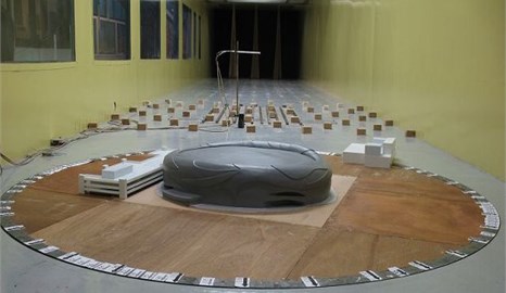
Fig. 3Mean wind speed and turbulence intensity profiles

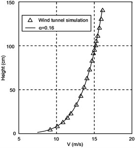
a) Mean wind speed profile

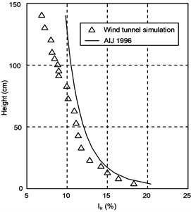
b) Turbulence intensity profile

This terrain type specifies a mean wind speed profile with a power law exponent of $α =$ 0.16. The measured mean wind speeds and turbulence intensities at various heights over the test section are illustrated in Fig. 3(a) and Fig. 3(b), respectively. Meanwhile, the turbulence intensity profile specified in the Japanese Load Code [28] is also shown in Fig. 3(b) for comparison purposes. The spectrum of longitudinal wind speed at the height of 45 m (0.225 m above the wind tunnel test section table) is shown in Fig. 4, which agrees with the von Karman spectrum well.

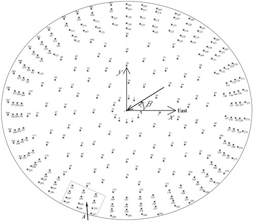
In fact, only the upper surface of the GISA roof is exposed to wind actions. Therefore, in order to obtain the wind pressures on the upper surface of the roof, 307 pressure taps were installed on its surface, which are marked with $\otimes$ shown in Fig. 5, for the pressure measurements. The layout of the pressure taps on the upper roof surface is shown in Fig. 5.

Fig. 4Spectra of longitudinal wind velocity at the height of 45 m in full-scale

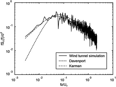
Fig. 5Layout of the pressure taps on the upper roof surface

2.3. Pressure measurements and data analysis

In the wind tunnel tests, pressures were measured simultaneously from all the taps on the upper roof surface, and data sampling frequency was 312.5 Hz with sampling length of 20480. Wind direction was defined as an angle $β$ starting from the east with anti-clockwise direction, thus $β$ varied from 0° to 360° with incremental step of 10°, as shown in Fig. 5.

The pressure measurements were carried out at a wind velocity with $U_{r e f} =$ 11.37 m/s at a reference height with $z_{r e f} =$ 60 cm. The pressure coefficient of the pressure tap $i$ on the roof surface is defined as follows:

1

C_{p i} (t) = \frac{p_{i} (t) - p_{\infty}}{p_{0} - p_{\infty}},

where $p_{i} (t)$ is the measured surface pressure at Tap $i$ ; $p_{0}$ and $p_{\infty}$ are the total pressure and the static pressure at the reference height, respectively.

The design wind speed with 100-year return period for GISA is about 47.06 m/s at the height of 120 m. Therefore, the velocity scale in the wind tunnel test is 1/4.14; and the time scale becomes 1/48.31. Then, the sampling frequency and the record length $T_{t o t a l}$ for the tested building are 6.47 Hz and 52.75 minutes in full scale, respectively. The period for evaluating the statistics of pressure fluctuations is specified as 10 min, which is usually used for the averaged time in wind speed measurements in China. The record time is divided into consecutive 10 min periods and the pressures at Tap $i$ are analyzed as mean, rms, maximum and minimum pressure coefficients, $C_{p i m e a n}$ , $C_{p i r m s}$ , $C_{p i m a x}$ and $C_{p i m i n}$ for each period. The averaged values from these five groups’ data are used in the following analysis. The wind tunnel experimental results indicate that the wind loads on the large-span roof structure are mainly dominant by relatively high negative wind pressures. Therefore, the peak factor, $g$ , corresponding to the minimum pressure coefficient can be defined as follows:

2

g = |\frac{C_{p m i n} - C_{p m e a n}}{C_{p r m s}}| .

3. Numerical simulation

By taking the GISA roof as an example, the present work mainly focuses on the development of an effective tool to accurately estimate the time series of wind-induced pressures in the unresolved area of long-span roof structure by neural network prediction method. There are a diverse range of neural networks, such as multilayer perceptron networks, Carpenter networks and Hopfield networks etc. The feedforward multilayer neural networks using a backpropagation training algorithm (BPNN) is probably the most widely used ANNs because of its proven performance for functional approximations, optimization and classification, etc. [36]. On the other hand, fuzzy system based on the pioneering work of Zadeh [9] in fuzzy set theory has been an active research area with wide applications in civil engineering such as earthquake intensity evaluation. However, a literature search indicates that generally the previous applications of ANNs or FNNs to wind engineering have concentrated their studies on the predictions of pressure coefficient distributions over various building models, but the usage of the ANN or FNN method to predict wind-induced pressure time series on buildings and structures has received little attention in the past.

Some further research studies [13] have shown that FNN approach has better convergence ability and impending speed than the BPNN approach in predicting the mean and RMS coefficient of wind-induced pressure on large roof structures. In other words, the FNN approach seems to be easier in training than the BPNN approach. FNN yields better prediction performance than the BPNN. The reason for this may be attributed to the fuzzy systems of the FNN. As the fuzzy systems in the FNN can convert the seeming irregular training data into an acceptable form using the membership function and $k$ -mean clustering technique [10], and then obtain proper fuzzy rules from the training data. In fact, the input of the FNN is the result of fuzzification with the obtained fuzzy rules, thus the FNN has stronger ability to capture the underlying nonlinear relationships than simplex BPNN. As a result, the FNN can produce more accurate results than the BPNN. Therefore, by taking the GISA roof as an example, this study adopted FNN method for the prediction of the time series of wind-induced pressure on the large-span roof structure on the basis of wind tunnel pressure measurements.

3.1. Fuzzy neural networks (FNN)

The topology of the fuzzy neural network (FNN $n$ - $m \cdot n$ - $m$ - $o$ ) used in the present research is shown in Fig. 6, which is comprised of four different layers: an input layer, a membership layer, an inference layer and a defuzzification layer (an output layer). The network consists of $n$ input variables with $n$ neurons in the input layer, $o$ output variables with $o$ neurons in the output layer, and $m$ number of rules with $m$ neurons in the inference layer; thus the number of neurons in the membership layer is $n$ × $m$ . However, for a given network structure, the numbers of neurons in the hidden layers can significantly affect the prediction performance of the FNN [7]. If there is insufficient number of hidden nodes, it may be difficult to reach convergence during the training process, as the network may be unable to create adequately complex decision boundaries. On the other hand, if too many hidden nodes are used, the network may lose its ability to be generalized; in addition, keeping the number of hidden layer nodes to a minimum reduces the number of weights that need to be adjusted, and hence reduces the computational time needed for training [37]. Therefore, in this study, several four-layer network structures with different numbers of hidden neurons have been considered by using a trial-and-error approach [7, 29] which starts with a small number of hidden neurons and then increasing the size until the training performance is acceptable. In this way $m$ can be generated by using $k$ -mean clustering technique [10], of course, the values of $m$ can also be adjusted with practical requirements.

Fig. 6Topology of the four-layer fuzzy neural network (FNN n-m⋅n-m-o)

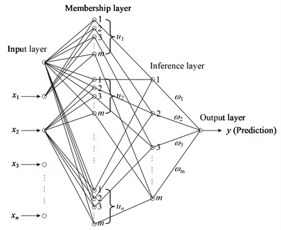
In the membership layer, each node performs a membership function, and the activation function of $u_{i}$ consists of a set of membership functions, i.e., $u_{i} = (u_{i 1}, u_{i 2}, \dots, u_{i m})$ . The Gaussian function is adopted as the membership function. For the $j$ th node of $u_{i}$ :

3

u_{i j} = e x p (- \frac{(x_{i} - m_{i j})^{2}}{σ_{i j}^{2}}), 1 \leq i \leq n, 1 \leq j \leq m,

where $u_{i j}$ is the value of the fuzzy membership function of the $i$ th input variable $x_{i}$ corresponding to the $j$ th rule; $m_{i j}$ and $σ_{i j}$ are, respectively, the mean and standard deviation of the Gaussian function in the $j th$ term of the $i th$ input variable $x_{i},$ and $m_{i} = (m_{i 1}, m_{i 2}, \dots, m_{i m}),$ $σ_{i} = (σ_{i 1}, σ_{i 2}, \dots, σ_{i m})$ .

The activation function in the inference layer uses multiplicative inference. For the $i$ th rule node, the output is given by:

4

π_{i} = u_{1 i} \times u_{2 i} \times \dots \times u_{n i} = \prod_{j = 1}^{n} u_{j i}, (1 \leq i \leq m) .

The defuzzification layer has the connecting weights ( $ω_{i}$ ) to the output from the inference layer, and these weights signify the strength of each rule in the output of the model. The output $y$ is given as:

5

y = ω_{1} π_{1} + ω_{2} π_{2} + \dots + ω_{m} π_{m} .

The learning algorithm [10] which is based on the conventional backpropagation neural network algorithm [29] was adapted herein to train the network, which aims to minimize the sum of the square errors. The square error is defined as:

6

E_{p} = \frac{1}{2} (y - Y)^{2},

where $y$ is the model output (prediction), $Y$ is the desired output (target).

According to the gradient descent method [29], the weights in the output layer are updated by the following equation:

7

ω_{i} (n + 1) - ω_{i} (n) = - η \frac{\partial E_{p}}{\partial ω_{i}},

where $η$ is the learning rate parameter of the weights and is a positive constant to be determined.

The update laws of $m_{i j}$ and $σ_{i j}$ can also be obtained by the gradient decent method, i.e.:

8

m_{i j} (n + 1) - m_{i j} (n) = - η \frac{\partial E_{p}}{\partial m_{i j}},

9

σ_{i j} (n + 1) - σ_{i j} (n) = - η \frac{\partial E_{p}}{\partial σ_{i j}} .

Here, assuming the learning-rate parameters of the mean and standard deviation of the Gaussian function are also $η$ .

Then, substituting Eqs. (7)-(9), respectively, into Eq. (6), the following equations are obtained:

10

ω_{i} (n + 1) - ω_{i} (n) = - η (y - Y) π_{i},

11

m_{i j} (n + 1) - m_{i j} (n) = - η (y - Y) ω_{j} \prod_{l = 1, l \neq i}^{n} u_{l j} 2 \frac{x_{i} - m_{i j}}{σ_{i j}^{2}} e^{- \frac{(x_{i} - m_{i j})^{2}}{σ_{i j}^{2}}},

12

σ_{i j} (n + 1) - σ_{i j} (n) = - η (y - Y) ω_{j} \prod_{l = 1, l \neq i}^{n} u_{l j} 2 \frac{(x_{i} - m_{i j})^{2}}{σ_{i j}^{3}} e^{- \frac{(x_{i} - m_{i j})^{2}}{σ_{i j}^{2}}} .

More detailed descriptions of the FNN can be found in Wang [10]. MATLAB and C based computer programs were made to develop the FNN model for the prediction of the time series of wind pressures on the GISA roof.

3.2. Prediction of wind pressure time series on the roof

In this study, the FNN predictions are presented for wind pressure time series at representative tap locations in zone $A$ at wind direction of 260° (see Fig. 5). The zone $A$ was chosen because this area is suffered by large pressure variations with high rms values; and large suctions often occur in this region due to strong flow separation at the leading edge in this wind direction [30-32]. Therefore, the prediction of the wind pressure time series in this area is expected to be difficult by conventional theoretical or numerical methods because of imperfect knowledge about the structure of separating/reattaching flows and their sensitivity to incident flow characteristics. It is expected that it is ideal for adopting FNN to learn the underlying nonlinear behavior by training the input-output data. Having learned the complex behavior, the captured functional relationship should be able to accurately predict the wind pressure time series at other locations if the underlying physical process governing the pressure time series does not change.

The available experimental data were allocated into two subsets: training data and testing data. The training data which consist of the experimental input-output data pairs at the wind directions of 260° in the zone $A$ (except the interpolation tap 196 and the extrapolation tap 289), were used to train the FNN. The remaining experimental data which were not used in the training were chosen as the new test data to evaluate the prediction accuracy of the developed FNN model. In other words, the developed FNN model will be used to predict the wind pressure time series at the two pressure taps (Nos. 196 and 289) under the wind direction of 260°. As we know, the time history datum for the pressure coefficient of taps on the long span roof structure are mainly determined by the approaching wind direction, the specified time instant and the spatial three-dimension coordinate data. The purpose of adopted FNN method in this study is to predict the time history of pressure coefficient $C_{p} (t)$ at the unresolved areas in the wind tunnel test. Therefore the number of neurons in the input layer for FNN method is selected as the value of 4. Totally 4 neurons including time instant ( $t$ ) and positions of pressure taps ( $x$ , $y$ , $z$ ) were considered as input variables in the FNN, and output variable(s) was the pressure coefficient $C_{p} (t)$ at the time instant $t$ . Thus the number of neurons in the output layer in FNN method is 1.

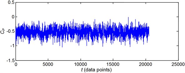
Fig. 7Comparison of pressure time series between the experimental data and the FNN prediction for pressure tap 196

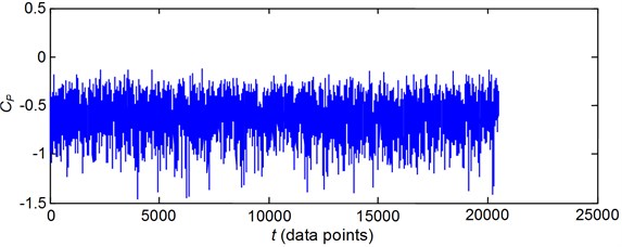
a) Experimental data

b) FNN prediction

For the FNN approach, the number of fuzzification and de-fuzzyfication rules, $m$ , for the samples of $C_{p} (t)$ , can be determined as 10 using the $k$ -mean clustering technique [10, 13] to cluster the samples of $C_{p} (t)$ . However, to obtain a faster training speed and higher prediction performance, several four-layer network structures with different numbers of rules, $m$ , which starts with 10 and then increasing the size until the training performance is acceptable, have also been considered. Finally it was found that the topology of the four-layer fuzzy neural network FNN 4-4×12-12-1 with $m =$ 12 has the best performance to predict the wind pressure time series.

Meanwhile the activation function in the membership layer adopts the Gaussian function. For the $i$ -th input variable $x_{i}$ corresponding to the $j$ th rule in the membership layer, the Gaussian function is defined by Eq. (3). The activation function in the inference layer uses multiplicative inference as defined in Eq. (4). By connecting weights to each output from the inference layer, the output of the defuzzification layer could be constructed.

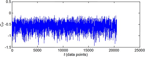
After training the FNN with the input-output example patterns, given the values of the input variables ( $x$ , $y$ , $z$ , $t$ ) from the testing data, the corresponding output, $C_{p} (t)$ at the time instant $t$ , can be obtained. In this way, the pressure coefficient at any time instant can be predicted. Thus, the whole time series can be predicted from the training data. Figs. 7 and 8 show comparisons of pressure time series between the experimental data and the FNN predictions for the previously “unseen” pressure taps 196 (the interpolation tap) and 289 (the extrapolation tap), respectively. Some results are summarized in Table 1, where the mean, rms, maximum and minimum pressure coefficients of the predicted and experimental time series data are compared.

Fig. 8Comparison of pressure time series between the experimental data and the FNN prediction for pressure tap 289

a) Experimental data

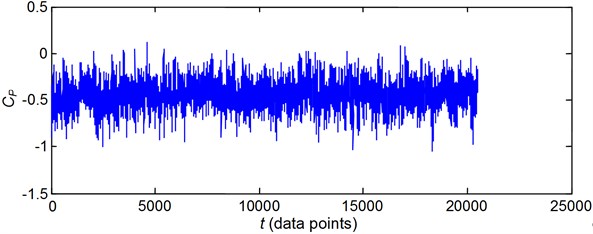
b) FNN prediction

Comparing the two time series of wind-induced pressures shown in Figs. 7 and 8, it is clear that the predicted time series for the two taps are both in a good agreement with the experimental data. This is demonstrated by the absolute values of the absolute errors, as shown in Table 1, between the experimental data and the FNN predictions, which are all close to 0. It can also be observed from Table 1 that the absolute values of the absolute errors and relative errors between the experimental data and the FNN predictions for the interpolation case (No. 196) are smaller than those for the extrapolation case (No. 289). This indicates that the prediction performance of the FNN for the interpolation case is better than that for the extrapolation case. The observed phenomenon can be explained as follows. Generally, for the interpolation case, the generalization domain of a given neural network model is the domain in the input space, where the model is applicable and good performance of the model can be expected. But for the extrapolation case, the generalization domain of the model is out of the input space, the performance of the model may deteriorate in the extrapolation domain [33]. As a result, the generalization ability of the neural network models for the interpolation case is superior to the result for the extrapolation case. Therefore, in applying the neural network approach to predict wind pressures on a large-span roof, it is better to install as more pressure taps as possible at the edges of the model surfaces in order to predict the wind pressures on the entire roof following interpolation cases.

Table 1Comparison of the experimental data and the FNN prediction results

Cases	Pressure	Mean	Rms	Minimum	Maximum
Interpolation (Pressure tap 196)	Measured	–0.6308	0.1708	–1.3138	0.0523
Interpolation (Pressure tap 196)	FNN	–0.6337	0.1745	–1.3219	0.0608
Absolute error		0.0029	0.0037	0.0081	0.0085
Relative error		0.46 %	2.17 %	0.62 %	16.25 %
Extrapolation (Pressure tap 289)	Measured	–0.5360	0.1163	–1.0012	–0.0707
Extrapolation (Pressure tap 289)	FNN	–0.5480	0.1295	–1.0815	–0.0943
Absolute error		0.0120	0.0132	0.0803	0.0236
Relative error		2.24 %	11.35 %	8.02 %	33.38 %

4. Equivalent static wind load discussions

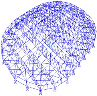
A three-dimensional finite element model of the roof structure of GISA was established based on the structural design drawings using a commercial computer package SAP2000, as shown in Fig. 9. The whole finite element model has 4270 nodes with 25620 degrees of freedom. The calculated results for the first 32 natural frequencies listed in Table 2 indicate that the natural frequencies of the GISA roof are very closely spaced, suggesting that the modal response correlations may be significant. Therefore, the modal response correlations should be taken into consideration in the wind-resistant design of such large-span roof structure; neglecting them will result in underestimated responses [34]. In the following analysis, the GISA roof is considered as an example to illustrate the application and effectiveness of the ESWL approach proposed by the authors [25]. The wind loading inputs acting on each node of the GISA roof in the finite element simulation are derived based on the multiple point simultaneous pressure measurements on the rigid roof model in conjunction with the FNN method presented in Section 3; and the damping ratio for each mode is assumed to be 2 % in this study.

Table 2The calculated results for the first 32 natural frequencies

Mode	$f$ (Hz)	Mode	$f$ (Hz)	Mode	$f$ (Hz)	Mode	$f$ (Hz)
1	1.5391	9	2.3033	17	2.5709	25	2.8241
2	1.6724	10	2.3165	18	2.6756	26	2.8464
3	1.8502	11	2.3190	19	2.6849	27	2.8544
4	2.0181	12	2.3531	20	2.7378	28	2.9048
5	2.1191	13	2.4247	21	2.8208	29	3.1480
6	2.1703	14	2.4721	22	2.8231	30	3.1536
7	2.2816	15	2.4847	23	2.8234	21	3.1817
8	2.3032	16	2.5246	24	2.8238	32	3.2552

4.1. Wind-induced response analysis

As mentioned in Fu et al. [25], using the random vibration theory and the CQC approach, wind-induced displacement responses of large-span roof structures can be determined; in which the contributions of higher modes and modal response correlations are taken into consideration for the estimated wind-induced responses. In general, the displacement responses of large-span roof structures due to wind excitation are mainly dominant in the vertical direction. When the incident wind direction varies from 0° to 360° with an incremental of 10°, there should be a node with the largest peak displacement response in $z$ -direction; and the critical wind direction is found to be an oblique angle ( $β =$ 320°) . Figs. 10(a)-(c) show the contour distributions of mean, RMS and peak displacement responses of the roof at the critical wind direction, respectively. It should be pointed out that the RMS displacement responses in Fig. 10(b) are calculated by the CQC approach, and not estimated by combining with the separated background and resonant response components.

Fig. 9Finite element model of the roof structure of GISA

It can be seen from Fig. 10 that the maximum values of mean, RMS and peak displacement responses are 6.8 mm, 0.8 mm and 10.0 mm, respectively. This indicates that the proportion of the RMS displacement response multiplied by the corresponding peak factor to the total peak displacement response is about 32 %. The results clearly demonstrate the importance of considering the influence of fluctuating wind for accurate predictions of wind effects on large-span roof structures.

4.2. A discussion of correlation between background and resonant response

However, in order to simplify the calculation, the RMS response is generally separated into the background and resonant components. The RMS response is estimated as the square root of the sum of the square of the background and resonant responses, which is expressed as:

13

σ = \sqrt{σ_{b}^{2} + σ_{r}^{2}},

where $σ_{b}$ and $σ_{r}$ are the background and resonant responses, respectively.

Or the peak response (with the mean response excluded) is obtained by combining the background and resonant components [35]:

14

R_{m a x} = \sqrt{g_{b}^{2} σ_{b}^{2} + g_{r}^{2} σ_{r}^{2}},

where $g_{b}$ and $g_{r}$ are peak factors for the background and resonant responses, respectively.

The separation strategy has the advantage of demonstrating the relative significance of the two components in the total RMS response; it can also provide a more efficient response prediction framework and a physically more meaningful description of loading distribution. But the correlations between the background and resonant components may be neglected, which would result in considerable error in the RMS response estimation.

Fig. 10Contour distributions of mean, RMS and peak displacement responses of the roof under a wind direction of 320° (unit: mm)

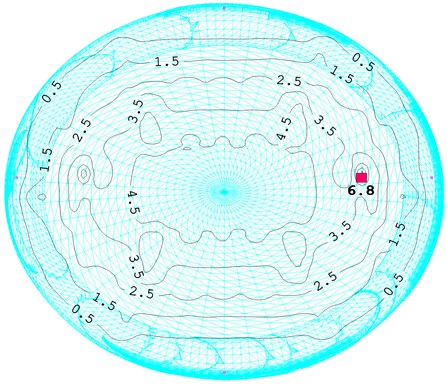
a) Mean displacement responses

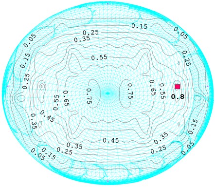
b) RMS displacement responses obtained by the CQC approach

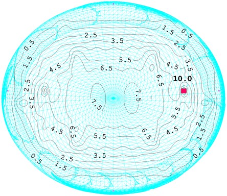
c) Peak displacement responses

As is well known, the wind-induced background and resonant responses are two random variables. Generally, the variables are not fully independent. Hence, in order to obtain more accurate results, the following equation should be adopted:

15

σ^{2} = σ_{b}^{2} + σ_{r}^{2} + 2 σ_{b} σ_{r} ρ_{b r},

where $ρ_{b r}$ is the correlation coefficient between the background and resonant components.

Obviously, the correctness of Eq. (13) or Eq. (14) is assured only if the correlation coefficient $ρ_{b r}$ equals zero. Otherwise, the results obtained from Eq. (13) or Eq. (14) are approximate values. The precision of Eq. (13) can be evaluated by the relative error which is expressed as:

16

e = \frac{σ - \sqrt{σ_{b}^{2} + σ_{r}^{2}}}{σ} .

A positive valued indicates that Eq. (13) yields underestimation of the response while a negative value indicates overestimation of the response. The GISA roof is illustrated here for the investigation of whether it is adequate to ignore the correlations for estimation of the wind-induced responses of large-span roof structures.

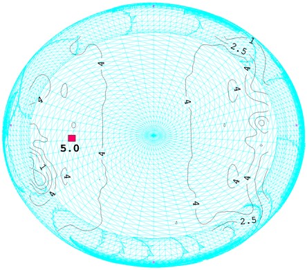
Figs. 11(a) and (b) show the contour distributions of background and resonant responses of the roof in wind direction of 320°, respectively. Based on Eq. (13), the overall RMS wind-induced responses can be estimated as the square root of the sum of the square of the background and resonant responses; and the corresponding contour distributions on the roof are plotted in Fig. 11(c).

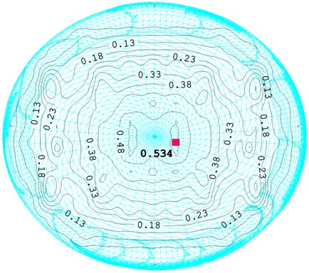
Furthermore, the distributions of correlation coefficients between the background and resonant response components on the whole roof structure are displayed in Fig. 12(a), and the associated relative errors are shown in Fig. 12(b). It can be seen from Figs. 12(a) and (b) that the maximum values of the correlation coefficients and relative errors are about 19.2 % and 5 %, respectively. This illustrates that the wind-induced response may be underestimated by up to 5 % when Eq. (13) is adopted for evaluation of the wind-induced displacement response. Such an error may not be neglected in the wind-resistant design of the large-span roof structure.

The above example clearly demonstrates that it is important to include the correlation coefficients between the background and resonant components in the estimation of wind-induced responses and ESWLs for large-span roof structures.

4.3. Comparison of the displacement response results from the CQC and ESWL approaches

Using the ESWL approach proposed by the authors [25], the ESWL for any peak displacement response can be conveniently determined by utilizing a static analysis approach and the CQC rule for the applications to the design of large-span roof structures.

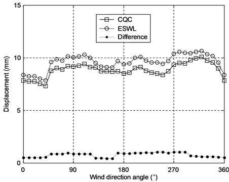
When the incident wind direction varies from 0° to 360° with an incremental of 10°, there should be a node of the finite element model with the largest positive or negative peak displacement response under each wind direction. The peak displacement responses of the above-mentioned nodes in $z$ -direction, obtained from the CQC and ESWL approaches, are plotted versus various incident wind directions in Fig. 13. It can be seen from this figure that the peak displacement responses determined from the ESWL approach are in a excellent agreement with those from the CQC approach. This can be shown from the absolute differences between the two sets of computational results, as shown in Fig. 13. Where the average absolute difference is 0.7582 mm, and the corresponding average relative difference is 8.57 %. The agreement between the two sets of results shown in Fig. 13 is quite satisfactory, illustrating that the ESWL approach proposed by the authors [25] can provide satisfactory predictions for wind-induced responses of large-span roof structures and thus verifying the effectiveness of the methodology again.

Fig. 11Contour distributions of background, resonant and RMS responses (unit: mm)

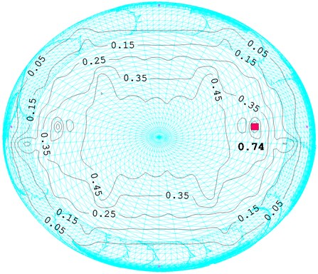
a) Background responses

b) Resonant responses

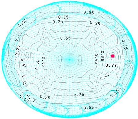
c) RMS displacement responses based on Eq. (13)

Fig. 12The correlations between background and resonant components and the associated relative errors

a) Correlation coefficients

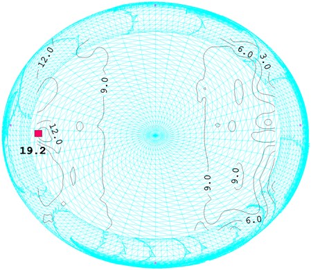
b) Relative errors

Fig. 13Comparison of the peak displacement responses from the CQC and ESWL approaches

5. Conclusions

This paper presents some selected results from a combined numerical simulation and ESWL study of wind effects on the GISA roof. Based on the pressure data measured from limited number of pressure taps, a numerical simulation approach using FNNs has been developed for the prediction of wind pressure time series at other roof locations which were not covered in the wind tunnel measurements. It was observed from this study that the FNNs have the potential to provide accurate predictions of wind pressure time series on the large-span roof structure. To the knowledge of the authors, the usage of the FNN method to predict time series of wind-induced pressures on buildings and structures has received little attention in the past.

On the other hand, the wind-induced response distributions on the roof are presented and discussed, which are directly calculated by the CQC approach and not separated into the background and resonant response components. Furthermore, the correlations between the background and resonant response components are discussed in detail, and the results show that neglecting the correlations between the two components would result in considerable error in the wind-induced response estimation. Finally, the peak displacement responses determined by the ESWL approach proposed by the authors [25] have been compared with those obtained from the CQC method, and it was found that the agreement between the two sets of results is quite satisfactory, thus verifying the accuracy of the proposed ESWL approach in the design and analysis of large-span roof structures. The accurate evaluation of the ESWL by the proposed approach for spatiotemporally varied wind loads is very attractive for simplifying the determination of design wind loads, which will be useful to aid in revising current design standards and codes to realistically predict wind effects on buildings and structures.

It is shown through the example that the FNN and ESWL approaches can successfully predict the wind-induced pressures and responses, respectively; and can serve as an effective tool for the design and analysis of wind effects on large-span roof structures in conjunction with wind tunnel tests.

References

Uematsu Y., Isyumov N. Wind pressures acting on low-rise buildings. Journal of Wind Engineering and Industrial Aerodynamics, Vol. 82, 1999, p. 1-25.

Search CrossRef
Ho T. C. E., Surry D. Factory mutual-high resolution pressure measurements on roof panels. The University of Western Ontario, Boundary Layer Wind Tunnel Laboratory Report: BLWT-SS11-2000, 2000.

Search CrossRef
Turkkan N., Srivastava N. K. Prediction of wind load distribution for air-supported structures using neural networks. Canada Journal of Civil Engineering, Vol. 22, 1995, p. 453-461.

Search CrossRef
Khanduri A. C., Bédard C., Stathopoulos T. Modelling wind-induced interference effects using backpropagation neural networks. Journal of Wind Engineering and Industrial Aerodynamics, Vol. 72, 1997, p. 71-79.

Search CrossRef
Sandri P., Mehta K. C. Using a backpropagation neural network for predicting wind induced damage to buildings. Proceedings of the Ninth International Conference on Wind Engineering, New Delhi, India, 1995, p. 1989-1999.

Search CrossRef
Chen Y., Kopp G. A., Surry D. Interpolation of wind-induced pressure time series with an artificial neural network. Journal of Wind Engineering and Industrial Aerodynamics, Vol. 90, 2002, p. 589-615.

Search CrossRef
Chen Y., Kopp G. A., Surry D. Prediction of pressure coefficients on roofs of low buildings using artificial neural networks. Journal of Wind Engineering and Industrial Aerodynamics, Vol. 91, 2003, p. 423-441.

Search CrossRef
Chen Y., Kopp G. A., Surry. D. Interpolation of pressure time series in an aerodynamic database for low buildings. Journal of Wind Engineering and Industrial Aerodynamics, Vol. 91, 2003, p. 737-765.

Search CrossRef
Zadeh L. A. Fuzzy sets. Information Control, Vol. 8, 1965, p. 338-353.

Search CrossRef
Wang S. T. Fuzzy Neural Systems and Their Applications. Beijing University of Aeronautics and Astronautics Publishing, Beijing, 1997, (in Chinese).

Search CrossRef
Lin S., Yang X. A fuzzy model for load combinations in structural analysis. Computers and Structures, Vol. 30, 1998, p. 999-1007.

Search CrossRef
Fu J. Y., Li Q. S., Xie Z. N. Prediction of wind loads on a large flat roof using fuzzy neural networks. Engineering Structures, Vol. 28, Issue 1, 2006, p. 153-161.

Search CrossRef
Fu J. Y., Liang S. G., Li. Q. S. Prediction of wind-induced pressures on a large gymnasium roof using artificial neural networks. Computers and Structures, Vol. 85, Issue 3-4, 2007, p. 179-192.

Search CrossRef
Chen X. Z., Kareem A. Equivalent static wind loads for buffeting response of bridges. Journal of Structural Engineering, Vol. 127, Issue 12, 2001, p. 1467-1475.

Search CrossRef
Kasperski M. Extreme wind load distributions for linear and nonlinear design. Engineering Structures, Vol. 14, 1992, p. 27-34.

Search CrossRef
Kasperski M., Niemann H. J. The LRC (load-response-correlation) method: a general method of estimating unfavorable wind load distributions for linear and nonlinear structural behavior. Journal of Wind Engineering and Industrial Aerodynamics, Vol. 43, 1992, p. 1753-1763.

Search CrossRef
Davenport A. G. The representation of the dynamic effects of turbulent wind by equivalent static wind loads. Proceeding of International Engineering Symposium on Structural Steel, Chicago, 1985, p. 1-13.

Search CrossRef
Irwin P. A. The Role of Wind Tunnel Modeling in the Prediction of Wind Effects on Bridges. Bridge Aerodynamics, Balkema, Rotterdam, The Netherlands, 1998, p. 59-85.

Search CrossRef
King J. P. C. Integrating wind tunnel tests of full aeroelastic models into the design of long span bridges. Proceeding of 10th International Conference on Wind Engineering, Copenhagen, 1999, p. 927-934.

Search CrossRef
Holmes J. D. Equivalent static load distributions for resonant dynamic response of bridges. Proceeding of 10th International Conference on Wind Engineering, Copenhagen, 1999, p. 907-911.

Search CrossRef
Holmes J. D. Effective static load distributions in wind engineering. Journal of Wind Engineering and Industrial Aerodynamics, Vol. 90, 2002, p. 91-109.

Search CrossRef
Holmes J. D., Kasperski M. Effective distributions of fluctuating and dynamic wind loads. Australian Civil Structural Engineering Transaction, Vol. 38, 1996, p. 83-88.

Search CrossRef
Zhou Y., Kareem A., Gu M. Equivalent static buffeting loads on structures. Journal of Structural Engineering, Vol. 126, Issue 8, 2000, p. 989-992.

Search CrossRef
Davenport A. G., King J. P. C. Dynamic wind forces on long span bridges. Proceeding of 12th International Association of Bridge and Structural Engineers Congress, Zurich, 1984.

Search CrossRef
Fu J. Y., Xie Z. N., Li Q. S. Equivalent static wind loads on long-span roof structures. Journal of Structural Engineering, Vol. 134, Issue 7, 2008, p. 1115-1128.

Search CrossRef
The Guangzhou International Sports Arena design narrative. MANICA Architecture, 2008.

Search CrossRef
GB50009-2001. Load code for the design of building structures. Architecture and Building Press of China, Beijing, 2002, (in Chinese).

Search CrossRef
AIJ Recommendations for Loads on Buildings. Architectural Institute of Japan, Japan, 1996.

Search CrossRef
Haykin S. Neural Networks: a Comprehensive Foundation. Macmillan Publishing, New York, 1999.

Search CrossRef
Li Q. S., Melbourne W. H. An experimental investigation of the effects of free-stream turbulence on streamwise surface pressures in separated and reattaching flows. Journal of Wind Engineering and Industrial Aerodynamics, Vols. 54-55, 1995, p. 313-323.

Search CrossRef
Li Q. S., Melbourne W. H. The effects of large scale turbulence on pressure fluctuations in separated and reattaching flows. Journal of Wind Engineering and Industrial Aerodynamics, Vol. 83, 1995, p. 159-169.

Search CrossRef
Li Q. S., Melbourne W. H. Turbulence effects on surface pressures of rectangular cylinders. Wind and Structures, Vol. 2, Issue 4, 1999, p. 253-266.

Search CrossRef
Pierre C. Three algorithms for estimating the domain of validity of a feedforward neural network. Neural Network, Vol. 7, Issue 1, 1994, p.169-174.

Search CrossRef
Chen X. Z., Matsumoto M., Kareem A. Aerodynamic coupling effects on flutter and buffeting of bridges. Journal of Engineering Mechanics, Vol. 126, Issue 1, 2000, p. 17-26.

Search CrossRef
Chen X. Z., Kareem A. Equivalent static wind loads for buildings: new model. Journal of Structural Engineering, Vol. 130, Issue 10, 2004, p. 1425-1435.

Search CrossRef
Bienkiewicz B., Ham H. J. Wavelet study of approach-wind velocity and building pressure. Journal of Wind Engineering and Industrial Aerodynamics, Vols. 69-71, 1997, p. 671-83.

Search CrossRef
Maren A., Harston C., Pap R. Handbook of Neural Computing Applications. Academic Press, San Diego, USA, 1990.

Search CrossRef
Smith D. A., Mehta K. C. Investigation of stationary and nonstationary wind data using classical Box-Jenkins models. Journal of Wind Engineering and Industrial Aerodynamics, Vol. 49, 1993, p. 319-28.

Search CrossRef
Huang Z., Chalabi Z. S. Use of time-series analysis to model and forecast wind speed. Journal of Wind Engineering and Industrial Aerodynamics, Vol. 56, 1995, p. 322-331.

Search CrossRef
Kumar K. S., Stathopoulos T. Computer simulation of fluctuating wind pressures on low building roofs. Journal of Wind Engineering and Industrial Aerodynamics, Vols. 69-71, 1997, p. 485-495.

Search CrossRef
Gurley K., Kareem A. Analysis interpretation modeling and simulation of unsteady wind and pressure data. Journal of Wind Engineering and Industrial Aerodynamics, Vols. 69-71, 1997, p. 657-669.

Search CrossRef
Dunyak J., Gilliam X., Peterson R., Smith D. Coherent gust detection by wavelet transform. Journal of Wind Engineering and Industrial Aerodynamics, Vol. 77-78, 1998, p. 467-478.

Search CrossRef
Aerospace Division of the American Society of Civil Engineers. Wind Tunnel Model Studies of Buildings and Structures, ASCE Manuals and Reports on Engineering Practice, No. 67.

Search CrossRef

About this article

Received

15 November 2014

Accepted

25 March 2015

Published

15 August 2015

SUBJECTS

Flow induced structural vibrations

Keywords

long-span steel structure roof

wind tunnel test

fuzzy neural network

equivalent static wind load

Acknowledgements

The work described in this paper was fully supported by grants from the National Natural Science Foundation of China (Project Nos. 51222801, 51378134), Yangcheng Scholarship in Guangzhou Municipal Universities (Project No. 12A004S) and the Research Funding for Ph.D. Programme in Higher Education Universities (Project No. 20124410110005). The financial supports are gratefully acknowledged.

This is an open access article distributed under the Creative Commons Attribution License, which permits unrestricted use, distribution, and reproduction in any medium, provided the original work is properly cited.