Abstract
This research proposed an eigen-assignment technique for locating and identifying structural damages using an incomplete measurement set. The sequential method is computationally efficient and requires no sensitivity calculations. Established by the finite element method, the mass and stiffness matrices are partitioned and measured partial eigenvectors are expanded to full modes. By matching calculated eigen-pairs with their measured counterparts as the termination criterion, the procedure solves for the stiffness reduction coefficients sequentially using a nonnegative least-squares solution scheme. The proposed approach can still find the damaged locations and the extent of the damage in a structure with much less measured degrees of freedom and even less measured modes than the finite element analysis degrees of freedom. The effectiveness of the technique is demonstrated by solving two cases based on a structure built for a benchmark study by the Group for Aeronautical Research and Technology in Europe (GARTEUR SM-AG19 structure).
1. Introduction
The purpose of structural nondestructive evaluation on a structure is to assess the structural integrity without removing individual components from it. For some structures, especially large and complex mechanical, aerospace and civil structures in operation, nondestructive evaluation may be the only choice to detect structural weakening or damage or any structural abnormality before a catastrophic structural failure may occur. For such structures, mathematical models derived from analytical approaches such as the finite element (FE) analysis are usually established in the design stage. The finite element models often require experimental verifications after the structures are constructed. If the analytical and the experimental results do not agree, the FE models can be tuned or updated to match the measured results [1-3]. An experimentally verified FE model provides a baseline that can be compared later with data collected from an in-service testing on the same structure to determine whether the structure is in a healthy condition. Damage in a structural member may be represented by a reduction in stiffness that consequently shifts the natural frequencies and changes the mode shapes of the original, undamaged structure. Alterations in measured frequencies and mode shapes indicate a faulty structure.
In recent years, many methods have been proposed to locate and assess structural damage from measured data. A direct, non-contact, acoustic-based damage detection method that was proposed by Arora et al. [4], used changes in vibro-acoustics flexibility matrices of the damage and health structure to detect the location and extend of structural damage. Instead of more traditional Euclidean norm minimization, Hernandez [5] presented a scheme utilizing norm minimization to solve the inverse problem of identifying localized damage. Noh et al. [6] introduced a sequential change-point diagnosis algorithm to perform a successive hypothesis test as a damage estimation procedure for civil structures. Cobb and Liebst [7] employed eigen-structure assignment in control theory to adjust an FE model to achieve the measured eigen-structure and thus to identify damage in a structure. The alternating projection method, which projects the undamaged FE stiffness matrix into a feasible matrix space constrained by positive semi-definiteness, symmetry, sparsity, and the eigen-equation constraints of the damaged structure, was proposed by Abdalla et al. [8]. Worden [9] used Artificial Neural Networks to construct the so-called novelty index to diagnose damage in mechanical systems. Lin [10] presented the concept of unity check and reduction coefficients to isolate damage suspected elements of an FE model.
In this study, a sequential eigen-assignment technique for locating and identifying structural damages using measured eigenvalues and partial eigenvectors is proposed. The mass and stiffness matrices of a finite element model for the intact (undamaged) structure are assumed to have been verified by a previous experimental modal testing. Also, the structural damage is assumed to be represented solely by stiffness reductions in the damaged structural members, which means that the mass distribution is not changed and that the mass matrices for the intact and damaged structures are the same. Unlike most methods depending on eigen-sensitivities to direct the searching process in a damage detection problem formulated as an optimization problem, the proposed method requires no sensitivity calculations. Instead, a partitioned form of the eigen-equation is used and measured partial eigenvectors are expanded to full modes. Then, a reduction coefficient for each finite element is defined and later found to indicate stiffness reduction in that particular element.
2. Structural damage identification procedure
An undamped, -DOF finite element model of an undamaged structure satisfies the following matrix form eigen-equation:
where and are the system stiffness and mass matrices, is the eigenvector matrix, and is the diagonal eigenvalue matrix. The eigenvector matrix also represents the structure’s mode shapes, and the eigenvalues in are squares of the natural frequencies. Assuming that the model has been verified by an experimental modal testing, the and matrices are known and they are considered as the baseline model. Further assuming that multiple structural damages can only cause stiffness reductions and no mass alterations, the damaged structure with damaged members at unknown locations and extents can be represented by and , which also satisfy the following equation:
where the superscript denotes the damaged state. In practice, not only is not known but also and cannot be measured entirely. In fact, the number of measured modes is much smaller than the system’s DOF. Denoting s as the number of measured modes, a truncated version of Eq. (2) can be written as:
in which is the truncated eigenvector matrix and is the corresponding eigenvalue matrix. Due to the fact that some locations of a structure may not easily assessable for mounting transducers and that rotational DOF are very difficult to measure, the size of each measured eigenvector is also smaller than that of its FE model counterpart. The truncated eigenvector matrix can be partitioned into an attained set (measured DOF, denoted by subscript ) and an omitted set (denoted by subscript ) as the following:
At this moment the attained portion of the truncated eigenvector matrix has a dimension of with being the number of measured DOF. The damaged stiffness matrix and the mass matrix can also be partitioned accordingly as:
Substitute the partitioned matrices into Eq. (3) and rearrange to give:
Rewrite Eq. (7) to yield:
Eq. (9) can be used to solve for the omitted parts of the eigenvectors as:
The full eigenvectors are then given as:
where:
and [] is the identity matrix. The truncated eigenvector matrix, the damaged stiffness and the mass matrices also satisfy the orthogonality equations as the following:
where the superscript denotes the transposing operator and is an diagonal matrix. The matrix is usually not an identity matrix since measured eigenvectors are not normalized with respect to the mass matrix. The damaged stiffness matrix is related to the intact one by:
where is the th element stiffness matrix, is the stiffness reduction coefficient for the th element, and is the total number of elements. For an undamaged structure, all reduction coefficients are zeroes, i.e. 0, 1, …, . Substitute Eqs. (16) and (17) into Eq. (15) to produce:
which can be rewritten as:
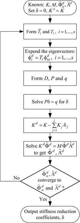
Fig. 1Flowchart of the identification procedure
The above matrix equation can be transformed into a standard form for an over-determined system of simultaneous equations as the following:
where:
and the operator is defined as stacking the diagonal and sub-diagonals of a matrix into a column vector. Although it’s not necessary to include the diagonal and all the sub-diagonals on the right hand sides of Eqs. (23) and (24), the number of terms should be so decided that Eq. (20) forms an over-determined system. However, more terms should increase statistical property of the solution. A least-squares solution to Eq. (20) can be obtained using the pseudo-inverse technique. Since the stiffness reduction coefficients are nonnegative, a better approach is to use a nonnegative least-squares solution scheme.
To implement the proposed method, first assign 0. Therefore, . The measured partial eigenvectors are expanded to full eigenvectors using Eq. (12) and then Eqs. (19) and (20) are formed. The solution of Eq. (20) provides an estimate for the stiffness reduction coefficient vector . At this stage, the first cycle of the procedure has now completed. Eqs. (16), (17) and (3) can be used to produce a pair of estimated eigenvector and eigenvalue matrices and then the measured eigen-pairs can be compared to see whether the process has converged. If not, Eq. (12) should be calculated instead and the process goes on to the next iteration. Fig. 1 depicts the flowchart of the proposed procedure for structural damage identification.
3. The GARTEUR SM-AG19 structure
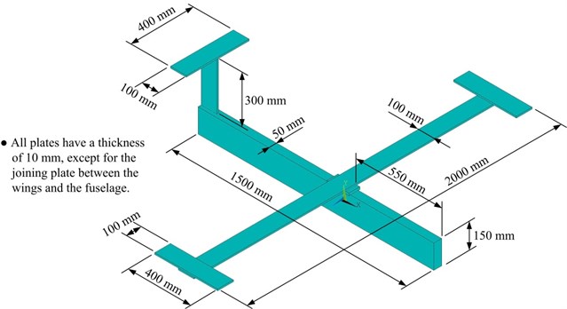
The proposed identification procedure will now be applied to the GARTEUR SM-AG19 structure [11-13], which was initially built for a benchmark study on experimental modal analysis conducted by the Structures and Materials Action Group (SM-AG) of the Group for Aeronautical Research and Technology in Europe (GARTEUR). The GARTEUR SM-AG19 structure, primarily made of one long Aluminum block as the fuselage and five Aluminum plates as the wings and vertical tail, has an overall length of 1.5 m with a wing span of 2.0 m (as shown in Fig. 2). The joining plate connecting the wings and the fuselage has a dimension of 140 mm×70 mm×15 mm.
Fig. 2Geometry of the GARTEUR SM-AG19 structure
The most commonly used finite element model for GARTEUR SM-AG19 is either a shell model [12] or a beam model [11, 13]. A 3D brick-element model and a simplified beam model is constructed using the software ANSYS (Fig. 3) and the results are compared in this study. The brick-element model has 5,324 SOLID186 elements with 21,992 nodes, and there are 102 BEAM188 elements with 103 nodes for the beam model. The material properties of both models are Young’s modulus 72 GPa, Poisson’s ratio 0.33 and mass density 2700 kg/m3.
Fig. 3a) 3D brick-element model and b) the beam model
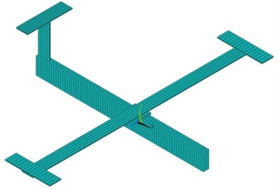
a)
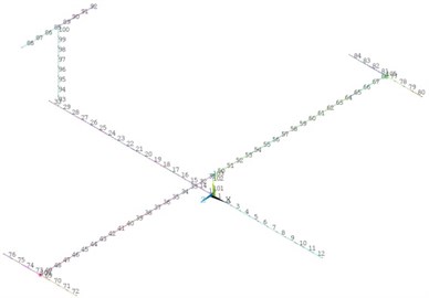
b)
Fig. 4Natural frequencies and mode shapes of the brick-element model in a free-free condition
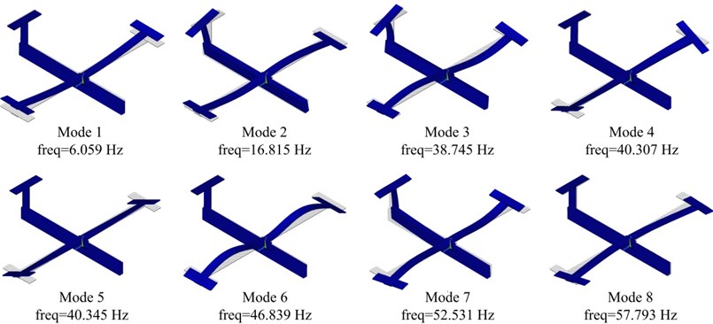
Fig. 5Natural frequencies and mode shapes of the beam model
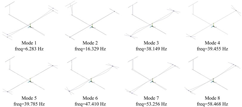
Fig. 4 shows the first 8 modes of the modal results for the brick-element model in a free-free boundary condition, excluding the rigid body modes. By applying the FE model updating technique on the beam model, which is carried out by adding and tuning one mass each at the fuselage-wing-joint node, the tail-tailplane-joint node and both wing-drum-joint nodes, the first 8 modes of the beam model shows a good correlation with those of the brick-element model, as shown in Fig. 5. The four added masses simulate the extra weights loaded on the beam model such as bolts, nuts, and joining plates and blocks.
4. Damage identification results and discussion
Since the prediction results of the beam model correspond very well with those of the brick-element model, the much simpler beam model is adopted to examine the effectiveness of the proposed identification procedure. Two cases with multiple damages are demonstrated in this study. Case 1 with two damaged elements (element no. 101 and no. 102), which are located at the fuselage-wing-joint and each has a Young’s modulus reduced to 80 % of the undamaged value, 72 GPa, can be seen in Fig. 6. A post-damage modal testing is conducted to obtain the damaged natural frequencies and mode shapes. The experimental case consists of strictly numerical simulation in which measurements are assumed taken only in the , and directions (no rotation DOF) at 54 measured nodes totaling to 162 measured DOF (see Fig. 6) and the number of measured modes is 20. The first ten natural frequencies of the intact and the damaged structures are compared in Table 1. As shown in Table 1, the frequency drops for the damage structure are not significant. In fact, there is one mode that has no change at all.
Fig. 6Damaged elements and the measured nodes for Case 1
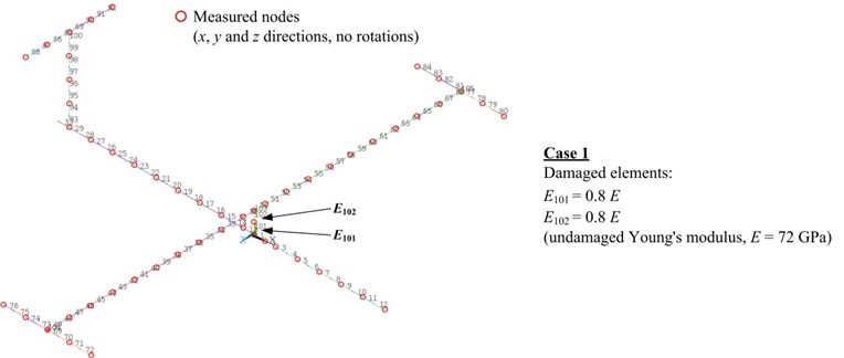
Table 1Comparison of natural frequencies for the intact and the damaged structures for Case 1
Mode number | Intact structure [Hz] | Damaged structure [Hz] | Frequency drop [%] |
1 | 6.283 | 6.282 | 0.016 |
2 | 16.329 | 16.327 | 0.012 |
3 | 38.149 | 37.339 | 2.123 |
4 | 39.455 | 39.036 | 1.062 |
5 | 39.785 | 39.785 | 0.000 |
6 | 47.410 | 47.371 | 0.082 |
7 | 53.256 | 52.137 | 2.101 |
8 | 58.468 | 58.436 | 0.055 |
9 | 63.492 | 63.490 | 0.003 |
10 | 72.457 | 71.075 | 1.907 |
The proposed method is applied to this damage detection problem according to the procedure stated earlier using the ANSYS APDL language and the MATLAB software. The solution to Eq. (20) is sought using the non-negative least-squares scheme. The iteration process converged very quickly in just 4 iterations and both damaged elements and the extent of their stiffness reductions are successfully identified. The stiffness reduction coefficients for element numbers 101 and 102 are both equal to 0.2, which means 0.8 and 0.8.
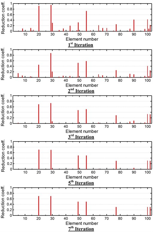
Case 2 with multiple damages in the beam model, which are shown in Fig. 7, are assumed to have defects in the elements with element numbers 20, 29, 49, 55, 77, 100 and 102 and their Young’s moduli are reduced to either 30 %, 50 % or 70 % of the undamaged value, 72 GPa. Again, 54 measured nodes with 162 measured DOF are attained and the number of measured modes is 20. The first ten natural frequencies of the intact and the damaged structures for Case 2 are compared in Table 2. The solution to Eq. (20) is sought repeatedly until convergence is achieved. The iteration process converges rather quickly and the iteration history and results are shown in Fig. 8. After only 7 iterations, all damaged elements and the extent of their stiffness reductions are clearly identified. The stiffness reduction coefficient for element no. 20, 0.7, for example, represents a 70 % decrease in Young’s modulus, i.e. 0.3.
Fig. 7Damaged elements and the measured nodes for Case 2
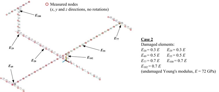
Table 2Comparison of natural frequencies for the intact and the damaged structures for Case 2
Mode number | Intact structure [Hz] | Damaged structure [Hz] | Frequency drop [%] |
1 | 6.283 | 5.326 | 15.232 |
2 | 16.329 | 14.200 | 13.038 |
3 | 38.149 | 33.612 | 11.892 |
4 | 39.455 | 34.459 | 12.662 |
5 | 39.785 | 38.947 | 2.161 |
6 | 47.410 | 42.446 | 10.470 |
7 | 53.256 | 50.083 | 5.958 |
8 | 58.468 | 56.062 | 4.115 |
9 | 63.492 | 60.857 | 4.150 |
10 | 72.457 | 67.971 | 6.191 |
The current method includes all elements in the damage detection process without isolating first a group of damage-suspected elements. If the number of elements of the FE model is large, it’s logical to localize a small area containing the damaged elements. Either the unity check procedure [10] or the strain energy method [14] may be employed to accomplish this task. When the number of damage-suspected elements, equivalent to the number of unknowns in Eq. (20), is reduced, the number of measured DOF can also be lessened.
Compared to sensitivity based methods, the proposed approach is easier to implement and requires less computer CPU time. Among the three methods of sensitivity calculations: the analytical, the semi-analytical, and the numerically approximated methods, the analytical one is most efficient. Although eigen-sensitivities have been analytically derived by several authors [15, 16], the finite difference scheme is more frequently chosen since analytical expressions of the eigen-sensitivities of a structure are often too complex to implement. For cases when eigen-sensitivities are approximated using finite differences, the saving of CPU time using the proposed method is even more significant.
Fig. 8Iteration results for damage identification of Case 2
5. Conclusions
In this paper, a computationally efficient damage identification procedure using measured partial eigenvectors and eigenvalues has been presented. The method assumes that damages in the structure cause only stiffness reductions in the damaged elements but do not alter the mass distribution of the structure. The method needs no sensitivity calculations and it can handle problems having much less measured DOF and eigen-modes than the finite element DOF. Two simulated cases, both converged very fast, have demonstrated the effectiveness of the procedure. The results have shown that damaged structural elements, represented by the stiffness reduction coefficients, can be located and the extent of their stiffness reductions can be determined in just a few iterations.
References
-
Chen K. N. Model updating and optimum designs for V-shaped AFM probes. Engineering Optimization, Vol. 38, Issue 7, 2006, p. 755-770.
-
Gant F., Rouch P., Louf F., Champaney L. Definition and updating of simplified models of joint stiffness. International Journal of Solids and Structures, Vol. 48, Issue 5, 2011, p. 775-784.
-
Gau W. H., Chen K. N., Hwang Y. L. Model updating and structural optimization of circular saw blades with internal slots. Advances in Mechanical Engineering, Vol. 2014, 2014, p. 1-11.
-
Arora V., Wijnant Y. H., de Boer A. Acoustic-based damage detection method. Applied Acoustics, Vol. 80, 2014, p. 23-27.
-
Hernandez E. M. Identification of isolated structural damage from incomplete spectrum information using l1-norm minimization. Mechanical Systems and Signal Processing, Vol. 46, 2014, p. 59-69.
-
Noh H., Rajagopal R., Kiremidjian A. S. Sequential structural damage diagnosis algorithm using a change point detection method. Journal of Sound and Vibration, Vol. 332, Issue 24, 2013, p. 6419-6433.
-
Cobb R. G., Liebst B. S. Structural damage identification using assigned partial eigenstructure. AIAA Journal, Vol. 35, Issue 1, 1997, p. 152-158.
-
Abdalla M. O., Grigoriadis K. M., Zimmerman D. C. Enhanced structural damage detection using alternating projection methods. AIAA Journal, Vol. 36, Issue 7, 1998, p. 1305-1311.
-
Worden K. Structural fault detection using a novelty measure. Journal of Sound and Vibration, Vol. 201, Issue 1, 1997, p. 85-101.
-
Lin C. S. Unity check method for structural damage detection. Journal of Spacecraft, Vol. 35, Issue 4, 1998, p. 577-579.
-
D’Ambrogioa W., Fregolent A. Dynamic model updating using virtual antiresonances. Shock and Vibration, Vol. 11, 2004, p. 351-363.
-
Link M., Friswell M. Working group 1: generation of validated structural dynamic models-results of a benchmark study utilising the GARTEUR SM-AG19 test-bed. Mechanical Systems and Signal Processing, Vol. 17, 2003, p. 9-20.
-
Salehi M., Ziaei-Rad S. Ground vibration test (GVT) and correlation analysis of an aircraft structure model. Iranian Journal of Science and Technology, Transaction B, Engineering, Vol. 31, Issue B1, 2007, p. 65-80.
-
Shi Z. Y., Law S. S. Structural damage localization from modal strain energy change. Journal of Sound and Vibration, Vol. 218, Issue 5, 1998, p. 825-844.
-
Dailey R. L. Eigenvector derivatives with repeated eigenvalues. AIAA Journal, Vol. 27, 1989, p. 486-491.
-
Nelson R. B. Simplified calculation of eigenvector derivatives. AIAA Journal, Vol. 14, 1976, p. 1201-1205.
About this article

