Abstract
A hybrid training method with probabilistic adaptive strategy for feedforward artificial neural network was proposed and applied to the problem of multi faults diagnosis of rolling bearing. The traditional training method such as LM shows fast convergence speed, but it’s easy to fall into local minimum. The heuristic method such as DE shows good global continuous optimization ability, but its convergence speed is slow. A hybrid training method of LM and DE is presented, and it overcomes the defects by using the advantages of each other. Probabilistic adaptive strategy which could save the time in some situation is adopted. Finally, this method is applied to the problem of rolling bearing faults diagnosis, and compares to other methods. The results show that, high correct classification rate were achieved by LM, and hybrid training methods still continued to converge while traditional method such as LM stopped the convergence. The probabilistic adaptive strategy strengthened the convergence ability of hybrid method in the latter progress, and achieved higher correct rate.
1. Introduction
Rolling bearings are one of the most widely used elements in machines and their failure is one of the most frequent reasons for machine breakdown. However, the vibration signals generated by faults in them have been widely studied, and very powerful diagnostic techniques are now available [1]. Early fault detection in rotating machineries is useful in terms of system maintenance and process automation, which will help to save millions on emergency maintenance and production costs [2]. Although the number of suitable techniques for bearing fault diagnosis increase when the more research works has been done, artificial neural networks is still one of the most effective approaches [3].
Artificial neural networks (ANNs) are important tools used in many areas such as regression, classification and forecasting [4]. And multi-layer feedforward networks is the most popular and widely used paradigm in many application [5]. The training methods of feedforward network include gradient decent method (GD) [6], conjugate gradient method (CG) [7], Levenberg-Marquardt method (LM) [8] etc. And some improved methods based on traditional methods are put forward to avoid slow convergence and being trapped in local minima [9, 10]. However, the number of suitable network training algorithms dramatically decrease when the neural network training becomes a large scale. Recently, the evolutionary artificial neural network (ANN) with heuristic training method attracts the interest of researchers [11]. However, in experiments of solving complicated problems, the convergence of the new method is not as good as some of the traditional methods [12].
In order to improve the convergence speed of EANNs, some research work combined heuristic training method with traditional training method like conjugate gradient method and LM method for training an artificial neural network are presented [13, 14]. LM method is a state-of-the-art method of traditional methods in ANN training, widely praised for its good convergence and easy implementation [15]. Differential evolution (DE) is one of the best heuristic methods for continuous global optimization [16]. By combining DE with LM, the hybrid method shows good global optimization ability as DE does, and shows good convergence as LM does [11]. In differential evolution, at the moment of starting, the differential term is very high. As the solution approaches to global minimum the differential term automatically changes to a low value. So during the initial period, the convergence speed is faster and the search space is very large, and it will increase the time used in a single iteration while individuals are trained second time by LM. And in LM, it requires more time to compute complex Jacobin matrix, and finish several times of network simulation.
In this paper, a probabilistic adaptive strategy is introduced in the hybrid training method, in which the LM is appropriately used according to the convergence speed of each individual and the population. It would reduce time used in a single iteration, improve the efficiency of the algorithm. First, time domain statistical characteristics and frequency domain statistical characteristics are calculated to form a feature set respectively. Then, single hidden layer ANNs classifiers are trained by the hybrid training method and other single training methods with the feature set. The proposed approach is applied to fault diagnosis of rolling element bearings. The vibration signals are collected from the rolling bearings under various operation loads and different bearing conditions. The results demonstrate the effectiveness of the proposed approach.
2. Feedforward ANNs and its training methods
Feedforward ANNs is one of the most popular artificial neural network, generally consists of an input layer, an output layer and several hidden layers. It has been proven that a network can approximate any continuous function to any desired accuracy [17]. And an ANN can solve a problem by using a single hidden layer as same as more hidden layers, provided it has enough number of neurons [18].
For units of hidden layer, the transfer function is generally logic or symmetric sigmoid function, and the symmetric sigmoid is more commonly used, and defined as:
For the units of the output layer, the transfer function is generally linear function, sometimes sigmoid or hard limit function.
2.1. Traditional training methods
The most common training method of the feedforward ANNs is gradient descent which performs steepest descent on a surface in weight space whose height at any point in weight space is equal to the error measure [3]. Gradient descent method is simple and easy to implement, it can be an efficient method for obtaining the weight values that minimize an error measure, and error surfaces frequently possess properties the make this procedure slow to converge. Several heuristics were proposed that provide guidelines for how to achieve faster rates of convergence than steepest descent techniques. Momentum implements the heuristics through the addition of a new term to the weight update equation [19]. A learning rate update rule that performs steepest descent on an error surface defined over learning rate parameter space implements the heuristics [20].
In most application of ANNs, there are often a large amount of weights need to be optimized. Although these algorithms based on the gradient descent are well known in optimization theory, they usually have a poor convergence rate and depend on parameters which have to be specified by the user. A quadratic convergent gradient method (Conjugate Gradient) is proposed to achieve faster convergence. The method is best able to deal with complex situations such as the presence of long curving valley. And the oscillatory behavior characteristic of methods such as steepest descents is thereby avoided [21].
The Levengerg-Marquardt algorithm is an approximation to Newton’s method. The key step in this algorithm is the computation of the Jacobian matrix. For the neural network mapping problem the terms in the Jacobian matrix can be computed by a simple modification to the backpropagation algorithm. And the LM algorithm can be considered a trust-region modification to Gauss-Newton, it is also easy to implement [5].
2.2. DE method
Differential evolutionary algorithm are used to perform various tasks, such as connection weight training, architecture design, learning rule adaption, and connection weight initialization from ANN’s, but mostly for connection weight training [22]. DE can be referred as heuristic optimization algorithms which are simple and intuitive, without a priori knowledge of the problem, and widely used in application. In [23], the differential evolution was first used to train the neural network, and got good convergence properties. The core process of DE contains three operations like GA, and they are mutation, crossover and selection [24].
The most common fitness function (or error function) is mean-square error (MSE), although in some situations other error criteria may be more appropriate [25]:
where constant is the length of output vector of the network, is the th parameter of target output vector, and is the th parameter of network output vector.
In [26], during experiments between variants of DE, DE/rand/1/either-or performs both fast and reliable. In which, the mutant vector is generated according to:
From experience can be recommended as a good first choice for given . Probability constant is introduced to implement a dual-axis search. The scheme accommodates functions above that are best solved by either mutation only (0) or recombination only (1), as well as generic functions that can be solved by randomly interleaving both operations (01).
3. Hybrid training method
The research work on evolutionary artificial neural network which is a special class of artificial neural network is still insufficient. On one hand, new efficient optimization techniques is developed on evolution algorithm and heuristic algorithm, etc. On the other hand, new training schemes are developed, and of which the hybrid training method has been studied lately.
The heuristic optimization techniques such as differential evolution are well known at their speed convergence and global optimization, and attract broad interest for application in many fields. However, some research works show that, while training much complex ANNs, the convergence speed of DE is not as good as some traditional method such as LM. But DE is more robust and not so easy to be trapped in local minimum that traditional methods always do.
Among all traditional training method of ANNs, LM method performs best at the convergence properties and global search abilities, is a state-of-the-art method in ANN training, but it also suffer from stagnation while being trapped in local minimum. A new training scheme combined LM method with DE method is proposed. The role of the DE here is to approach towards global minimum point and then LM is used to move forward achieving fast convergence. According to the proposed algorithm after reaching the basin of global minimum point the algorithm is switched from global search of the evolutionary algorithm (DE) to local search, LM [11]. As LM is a gradient based algorithm it can be exploited to increase the convergence speed for reaching the global minimum point.
3.1. Probabilistic adaptive strategy
The DE-LM algorithm that combined DE and LM is one of hybrid methods combined heuristic method with traditional method. It trains the target vector twice, first in the process of DE to reach a basin global minimum point, and then in the process of LM to increase the convergence. It shows that the hybrid method could well solve the complex problems like nonlinear system identification [11]. In the scheme, it needs more time to complete process from one generation to the next generation.
For most problems, the convergence speed of the DE is very high at the moment of starting, as the solution approaches to the global minimum the convergence speed automatically changes to a low value. Mention that the LM method is used to reach faster rate of convergence, so during the initial period, the process of LM method should not be proceeded, then the time used in a single iteration would be reduced. Furthermore, the decrease using LM method could reduce the risk that the population would be lead to a local minimum.
The convergence speed of the population is related to the convergence speed of all individuals in DE, because the fitness value of the population is the fitness value of the best individual of current iteration. Sometimes the individual with too fast convergence speed leads the entire population to a local minimum trap that hard to be escaped, because the individuals with low convergence speed would learning those with fast convergence speed. But it shows low convergence speed if there are too many low converged individuals in the population. So we want to enhance the convergence properties of those individuals with low convergence speed by using the LM method.
For each target vector of the th iteration, the fitness function is denoted by . The convergence speed of target vector and the population of the th iteration are denoted by and respectively:
where is a small positive number which ensures that is greater than 0. Namely, taken as the mean convergence speed of the population, so . Taken as the evaluation index of the convergence rate of the individual to the population.
With the increase of iteration, the convergence speed of individuals and the population changes to a low value, and during the later period it even stops change and the value is nearly equal to 0. Hence the mean convergence speed of the population will be far greater than the individuals because the mean convergence speed of the population is averaged by the speed of all the steps before, including the much greater ones during the initial period. Then the evaluation index is nearly 0. To this end, while it is evaluating the convergence rate of the individual, the mean convergence speed of the population is averaged only of several steps before. Assume the length of the evaluation steps is , then . Define event E: the target individual is second trained by LM method.
The probability of the event should be large, more close to 1, if the individual didn’t find better fitness value. This moment, the convergence speed of the individual is less than or equal to 0, and the mean convergence speed of the population is greater than 0, so the evaluation index is less than or equal to 0.
The probability of the event should be small, and close to 0, if the individual did find a better fitness value. This moment, the convergence speed of the individual is greater than or equal to 0, and the evaluation index is less than or equal to 0 too.
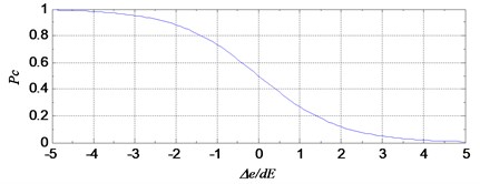
So we developed the following expression to set a value for each individual:
In the process of the algorithm, is used to generate a random real number from the interval [0, 1]. If , make the event become real, that means the target individual would be second time trained by LM method. Fig. 1 shows the relationship between the probability of event and the evaluation index of the individual.
Fig. 1The probability of the event E to the evaluation index
3.2. Proposed hybrid training algorithm
The proposed hybrid method combines DE with LM, using the probability adaptive strategy discussed above (DE-LM-PAS). In the process of the algorithm, the target vector is first trained by DE, the new generated target individual is then trained by LM according to the probability which is decided by the convergence speed of the individual and the population. After that, a new trial vector is obtained. The flow of the proposed method is presented:
Step 1: Initialize .
Step 2: , start the first iteration.
Step 3: , choose the first individual.
Step 4: Take the mutant, crossover and selection operations of the individual , generate the new individual of next generation and update the best individual .
Step 5: Evaluate the convergence speed of each individual and the mean convergence speed of the population, then evaluate the probability of each individual according to Eq. (5).
Step 6: Generate a random number . If , go to step 7, else continue.
Step 6.1: Calculate the Jacobian matrix of the individual .
Step 6.2: , where is the outputs of the network.
Step 6.3: Get the new trial vector .
Step 6.4: If the fitness value , then and continue to step 6.4.1, else go to step 6.4.2.
Step 6.4.1: If the fitness value , then and go to step 7.
Step 6.4.2: If , then and go to step 6.2.
Step 7: If , go to step 8, else and go to step 4.
Step 8: If a termination condition is reached, exit the loop, and go to step 9, else and go to step 3.
Step 9: Output the network with weight vector .
4. Fault diagnosis of rolling bearing
Rolling bearing is one of the most important elements of rotary machine, and most rotary machine failure is caused by rolling bearing faults. Hence, early bearing damage detection can significantly help reduce the costs that these downtimes will entail [27]. Statistical data show that approximately 90 % of rolling bearing failures are related to either inner race or outer race flaws, and the rest are related to rolling elements flaws [28]. In recent years, the problem of multi faults diagnosis attracts more and more research interests [29, 30].
The experiment data are obtained from the Case Western Reserve University Bearing Data Center [31]. The bearings used in this work are groove ball bearings manufactured by SKF. Reliance Electric’s 2-hp motor, along with a torque transducer, a dynamometer, and control electronics, constitutes the test setup. Fig. 2 shows experimental setup. The faults are introduced into the drive-end bearing of the motor using the electron discharge machining (EDM) method. The defect diameter of the three faults are the same: 0.18, 0.36 or 0.54 mm.
Fig. 2Experiments setup for vibration monitoring
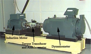
Table 1Description of data sets
Data set | Operating condition | Number of training samples | Number of testing samples | Defect diameter of fault point | Label of classification |
A | F0 | 30 | 30 | D0 | 1 |
F1 | 30 | 30 | D1 | 2 | |
F2 | 30 | 30 | D1 | 3 | |
F3 | 30 | 30 | D1 | 4 | |
B | F0 | 30 | 30 | D0 | 1 |
F1 | 30 | 30 | D1 | 2 | |
F2 | 30 | 30 | D1 | 3 | |
F3 | 30 | 30 | D1 | 4 | |
F1 | 30 | 30 | D3 | 5 | |
F2 | 30 | 30 | D3 | 6 | |
F3 | 30 | 30 | D3 | 7 | |
C | F0 | 30 | 30 | D0 | 1 |
F1 | 30 | 30 | D1 | 2 | |
F2 | 30 | 30 | D1 | 3 | |
F3 | 30 | 30 | D1 | 4 | |
F1 | 30 | 30 | D2 | 5 | |
F2 | 30 | 30 | D2 | 6 | |
F3 | 30 | 30 | D2 | 7 | |
F1 | 30 | 30 | D3 | 8 | |
F2 | 30 | 30 | D3 | 9 | |
F3 | 30 | 30 | D3 | 10 |
The shaft rotational speed of the rolling bearings is 1796 rpm. The data collection system consists of a high bandwidth amplifier particularly designed for vibration signals and a data recorder with a sampling frequency of 12,000 Hz per channel. In the present work, the original data set is divided into some signals of 2048 data points to extract features.
In order to evaluate the proposed method, three different data subsets (A-C) were formed from the whole data set of the rolling bearing. The detailed descriptions of the three data sets are shown in Table 1.
In the table, the four different operating conditions of the rolling bearings are denoted by F0-F3. F0: normal condition, F1: inner race fault, F2: outer race fault, F3: ball fault. The four different diameters of the fault point are denoted by D0-D3. D0: no fault points, D1: a fault point of 0.18 mm diameter, D1: a fault point of 0.36 mm diameter, D3: a fault point of 0.54 mm diameter.
Data set A consists of 240 data samples of normal condition and fault conditions with the defect size of D1. It is a four class classification task corresponding to the four different operating conditions, and it is not very difficult to take a high rate of correct classification.
Data set B contains 420 data samples of normal condition and fault conditions with the defect sizes of D1 and D3. It is a seven class classification that makes data set B is more difficult to be correctly classified than data set A.
Data set C comprises 600 data samples covering four different conditions. Each fault condition includes the three different defect diameters of D1-D3, respectively. Because it is a ten class classification problem and therefore very difficult.
4.1. Feature extraction
In order to reduce the error rate of classification of the bearing faults, features extracted must reveal enough information of the different types of faults. Hence, only some time-domain features are not enough, frequency-domain features that can reveal more fault information are needed [32]. In this paper, six time domain feature parameters and five frequency domain feature parameters are used for classification of the bearing faults. The difference of the feature values of the data is large, and the normalized treatment is carried out before using the data:
where is the extrated feature value and is the normalized feature value, and are the maximal and minimal feature values. From the table above, we know that data set C contains 600 samples, half of which are training samples and the rest are testing samples. Here, the 300 training samples of ten classes are used to extracted features. Here the samples are labled with number 1 to 600.
Table 2Ten classes of training and testing samples
Class | 1 | 2 | 3 | 4 | 5 | 6 | 7 | 8 | 9 | 10 |
Training samples | 1-30 | 31-60 | 61-90 | 91-120 | 121-150 | 151-180 | 181-210 | 211-240 | 241-270 | 271-300 |
Testing samples | 301-330 | 331-360 | 361-390 | 391-420 | 421-450 | 451-480 | 481-510 | 511-540 | 541-570 | 571-600 |
Fig. 3 shows the six time domain features (-). Most of the features show concentrated in class 1 to class 4, because the defect diameters of the samples of these classes are small, the amplitude and energy of the vibration signal are more steady. The features of class 7 to class 9 are more dispersed, and that makes it hard to identify the fault of same group correctly.
Single feature parameter can be used to identify the different class of samples, because it shows different values between different classes. The feature parameter are obviously different among class 1 to 3, but it almost shows the same value between class 1 and class 4, so the feature parameter can be used to distinguish the two class. Similarly, the feature parameter can be used to distinguish class 5 and class 6, can be used to distinguish class 6 and class 7, can be used to distinguish class 7 and class 8, and for class 8, class 9 and class 10. But while identifying class 7, class 8 and class 9, it is hard to get a high correct rate because of the dispersed feature values. And it is also difficult to identify the ten classes of samples with a high rate at the same time. So much more feature information needed.
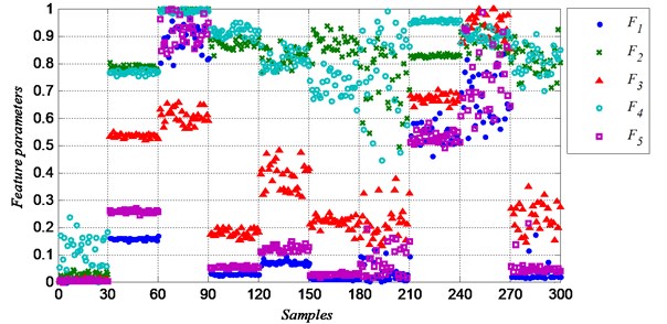
Fig. 4 shows the five frequency domain features (-). Obviously, the frequency domain features show more difference between groups, and less difference in a group than the time domain features. In class 8, all the time domain features show very dispersed, but the frequency feature and show very concentrated. By using the frequency domain feature, it would highly increase the classification correct rate. Both the time domain and the frequency domain feature values are more dispersed in a group when the defect diameter is bigger, especially in class 7 (ball fault with defect size of D2), class 9 (outer race fault with defect size of D3) and class 10 (ball fault with defect size of D3). Because the uncertainty increase while the fault is becoming worse. That makes it more difficult to classify the different conditions.
Fig. 3Normalized time domain feature parameters
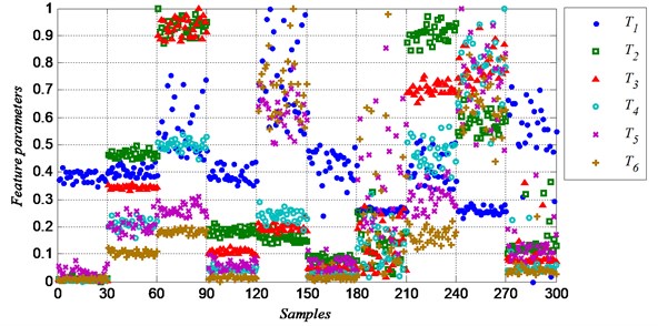
Fig. 4Normalized frequency domain feature parameters
4.2. Faults diagnosis
The multi-layer network classifiers are consists of three layers, the hidden layer contains 15 units, the input layer contains 11 units corresponding to the feature parameters, and the output layer contains units corresponding to the number of classes. The th output of the network is 1, and the rest output is 0 if the sample was labeled .
The single training methods contain gradient decent method (GD), scaled gradient method (SCG), Levenberg-Marquardt method (LM) and differential method (DE). The hybrid training methods contain the hybrid method of DE and LM with a simple strategy (DE-LM) and the hybrid method of DE and LM with a probability adaptive strategy (DE-LM-PAS). First, train the classifiers with the train sets, and then use these classifiers to identify the samples of train sets and test sets. The experiments repeat 10 times, and it stops when the number of net simulation reaches 104 or it meets other termination. The results show in Table 3.
Table 3Correct rate of classification (%)
Data set | GD | SCG | LM | DE | DE-LM | DE-LM-PAS |
Train/Test | Train/Test | Train/Test | Train/Test | Train/Test | Train/Test | |
A | 100/100 | 100/100 | 100/100 | 96.56/95.52 | 100/100 | 100/100 |
B | 91.95/92.81 | 94.29/94.67 | 99.71/99.24 | 70.00/68.93 | 100/99.33 | 100/99.57 |
C | 71.46/71.38 | 88.67/88.14 | 98.33/96.06 | 39.67/41.00 | 100/96.24 | 100/96.86 |
For data set A, it was not very difficult to solve a four class classification problem, classifiers with all train methods got a high correct rate on train set and test set, and all got a rate of 100 % except DE.
For data B, it was more difficult to solve a seven class classification problem. Only two methods got full correct rate of recognition in train set, and all methods performed worse in test set. In all methods, LM, DE-LM and DE-LM-PAS performed better with a high correct rate that is greater than 99 % in either train set or test set.
For data set C, it is very difficult to solve a ten class classification problem. GD, SCG and DE performed much worse than the rest three methods. And among worse methods, SCG was better than the other two methods. From the classification errors shown in Fig. 5, we can see that, the samples which were misclassified were almost from the groups of ball faults with defect sizes of D2 and D3. And the rest three better methods also performed on these samples of ball faults with defect sizes of D2 and D3. On the other fault samples, there were almost no errors as shown in Fig. 6.
Fig. 5Classification errors of GD, SCG and DE
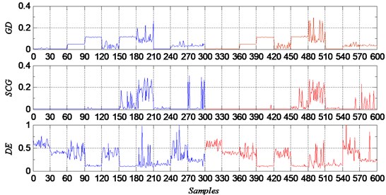
Fig. 6Classification errors of LM, DE-LM and DE-LM-PAS
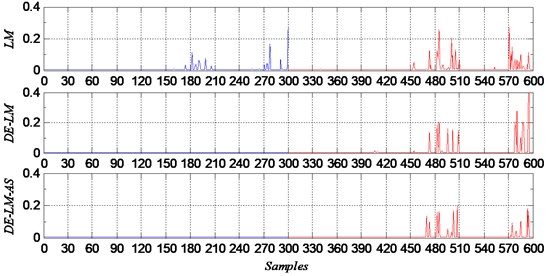
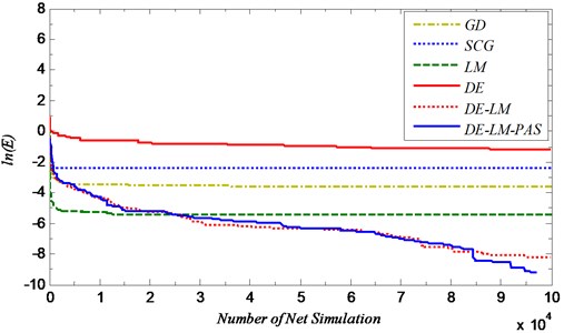
Fig. 7 shows the convergence curves of all methods. The three tradition methods GD, SCG and LM got a fast convergence rate during the initial period, but they stop to obtain a better value after 104th net simulations. However, DE and the hybrid methods could continue to converge during the whole process, but DE finally got a worse result because its convergence speed was slow.
Fig. 7Convergence curves of all method
4.3. Further experiments
In a realistic industrial environment, there is more noise in the signals. So more experiments are request to test how the proposed system operates when signals are embedded into the additive noise. In the experiments below, 20 % noise is added to the signals. Six time domain feature parameters and five frequency domain feature parameters are used, Fig. 8 shows the features extracted.
Fig. 8Features of the signals with 20 % noise
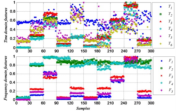
Fig. 8 shows that the time domain feature were infected badly with additive noise, but the frequency feature didn’t show much more different compared with the original signals. The classifiers are also trained by GD, SCG, LM, DE, DE-LM and DE-LM-PAS. The number of hidden layer units and the running options of each algorithm are same as the experiments before. The results show in Table 4.
Compared to the results in Table 3, the results are robust. The noise added into the signals did infect the correct rate of classification, but the infection is limited.
In a realistic industrial environment, the defect size is not just 0.18 mm, 0.36 mm or 0.54 mm, it could be any defect size. It is impossible to identify the uncertain defect size by using any classifiers. But the defect sizes could be clustered into several certain sizes like 0.18 mm, 0.36 mm, etc. If the signals exist difference between feature values, then the proposed system works, and the different faults could be recognized. Furthermore, the experiments above are all the early fault experiments, the defect sizes are relatively close. If differences exist in the feature values of the signals from the experiment, the differences also exist in a realistic industrial environment.
Table 4Correct rate of classification (%)
Data Set | GD | SCG | LM | DE | DE-LM | DE-LM-PAS |
Train/Test | Train/Test | Train/Test | Train/Test | Train/Test | Train/Test | |
A | 98.17/98.28 | 97.7/97.92 | 100/100 | 97.92/97.68 | 100/100 | 100/100 |
B | 91.36/91.04 | 92.24/92.09 | 99.17/99.04 | 67.73/69.87 | 100/99.17 | 100/99.49 |
C | 71.71/70.55 | 88.40/87.53 | 98.11/95.31 | 39.00/40.67 | 99.87/96.31 | 99.91/96.67 |
5. Conclusions
In this paper, a probability adaptive strategy hybrid training method of DE and LM for feedforward neural networks is proposed. It reduces the time for iterative process by probability adopting the hybrid training according to the convergence speed of the individuals and the population. The hybrid methods with simple strategy and probability adaptive strategy, and other single training methods are applied to the problems of rolling bearing multi fault diagnosis. The main conclusions are as follows:
1) Experiment results show that, the traditional methods are easy to be trapped in a local minimum and stop to converge, but they have a fast convergence speed during the initial period. However, differential evolutionary method with a low convergence speed can continue to converge during the whole period.
2) The hybrid training methods get the global optimization ability that is obtained from the differential evolutionary method, get the fast convergence ability is obtained from LM. The hybrid method overcomes the shortcomings of single training methods. It can continue to converge while the traditional method such as LM stop convergence, and performs fast convergence during the whole process.
3) Using the probability adaptive strategy, the hybrid method reduce some hybrid process, and avoid being trapped in local minimum because of too fast convergence. And it gets a better convergence speed during later period.
4) The network classifier trained by hybrid method with probability adaptive strategy can well solve the problem of multi faults diagnosis, and get a high correct recognition rate. Further experiments show that the classification results are robust when the signals are embedded into additive noise.
References
-
Randall R., Antoni J. Rolling element bearing diagnostics – a tutorial. Mechanical Systems and Signal Processing, Vol. 25, 2011, p. 485-520.
-
Raj A. S., Murali N. Early classification of bearing faults using morphological operators and fuzzy inference. IEEE Transactions on Industrial Electronics, Vol. 60, Issue 2, 2013, p. 567-574.
-
Lei Yaguo, He Zhengjia, Zi Yanyang, et al. Fault diagnosis of rotating machinery based on multiple ANFIS combination with GAs. Mechanical Systems and Signal Processing, Vol. 21, Issue 5, 2007, p. 2280-2294.
-
Ripley B. D. Pattern Recognition and Neural Networks. Cambridge University Press, Cambridge, 1996.
-
Paliwal M., Kumar U. Neural networks and statistical techniques: a review of applications. Expert Systems with Applications, Vol. 36, 2009, p. 2-17.
-
Rumelhart D. E., Hinton G. E., Williams R. J. Learning internal representations by error propagation. DTIC Document, 1985, p. 319-362.
-
Møller M. A scaled conjugate gradient algorithm for fast supervised learning. Neural Networks, Vol. 5, 1993, p. 525-533.
-
Hagan M., Menhaj M. Training feedforward networks with the Marquardt algorithm. Neural Networks, Vol. 5, Issue 6, 1994, p. 989-993.
-
Jacobs R. A. Increased rates of convergence through learning rate adaptation. Neural Networks, Vol. 1, 1988, p. 295-307.
-
Chang W. F., Mak M. W. Conjugate gradient learning algorithm for recurrent neural networks. Neurocomputing, Vol. 24, 1999, p. 173-189.
-
Yao X., Islam M. Evolving artificial neural network ensembles. Computational Intelligence Magazine, Issue 2, 2008, p. 31-42.
-
Ilonen J., Kamarainen J., Lampinen J. Differential evolution training algorithm for feed-forward neural networks. Neural Processing Letters, Vol. 17, 2003, p. 93-105.
-
Bandurski K., Kwedlo W. A Lamarckian hybrid of differential evolution and conjugate gradients for neural network training. Neural Processing Letters, Vol. 32, 2010, p. 31-44.
-
Subudhi B., Jena D. A differential evolution based neural network approach to nonlinear system identification. Applied Soft Computing, Vol. 11, 2011, p. 861-871.
-
Piotrowski A., Osuch M., Napiorkowski M., et al. Comparing large number of metaheuristics for artificial neural networks training to predict water temperature in a natural river. Computers and Geosciences, Vol. 64, 2014, p. 136-151.
-
Das S., Suganthan P. Differential evolution: a survey of the state-of-the-art. Evolutionary computation, Vol. 15, Issue 1, 2011, p. 4-31.
-
Zhang G., Patuwo B. E., Hu M. Y. Forecasting with artificial neural networks: the state of the art, International Journal of Forecasting, Vol. 14, 1998, p. 35-62.
-
Haykin S. Neural Networks: a Comprehensive Foundation. Prentice Hall, New York, 1999.
-
Plaut D. C., Nowlan S. J., Hinton G. E. Experiments on learning by back propagation. ERIC, Vol. 6, 1986.
-
Jacobs R. A. Increased rates of convergence through learning rate adaptation. Neural networks, Vol. 1, 1988, p. 295-307.
-
Fletcher R., Reeves C. M. Function minimization by conjugate gradients. The Computer Journal, Issue 7, 1964, p. 149-154.
-
Yao Xin. Evolving artificial neural networks. Proceedings of the IEEE, Vol. 87, Issue 9, 1999, p. 1423-1447.
-
Masters T., Land W. A new training algorithm for the general regression neural network. IEEE International Conference on Systems, Man, and Cybernetics. Computational Cybernetics and Simulation, 1997, p. 1990-1994.
-
Storn R., Price K. Differential evolution – a simple and efficient heuristic for global optimization over continuous spaces. Journal of Global Optimization, Vol. 11, 1997, p. 341-359.
-
Widrow B., Lehr M. A. 30 years of adaptive neural networks: perceptron, madaline, and backpropagation. Proceedings of the IEEE, Vol. 78, Issue 9, 1990, p. 1415-1442.
-
Price K., Storn R., Lampinen J. Differential evolution a practical approach to global optimization. Natural Computing, 2005, p. 135-156.
-
Zoubek H., Villwock S., Pacas M. Frequency response analysis for rolling-bearing damage diagnosis. IEEE Transactions on Industrial Electronics, Vol. 55, Issue 12, 2008, p. 4270-4276.
-
Bently D. Predictive Maintenance Through the Monitoring and Diagnosticsof Rolling Element Bearings. Bently Nevada Co., 1989, p. 2-8.
-
Abbasion S., Rafsanjani A., Farshidianfar A., et al. Rolling element bearings multi-fault classification based on the wavelet denoising and support vector machine. Mechanical Systems and Signal Processing, Vol. 21, 2007, p. 2933-2945.
-
Lei Yaguo, He Zhengjia, Zi Yanyang, et al. Fault diagnosis of rotating machinery based on multiple ANFIS combination with GAs. Mechanical Systems and Signal Processing, Vol. 21, Issue 5, 2007, p. 2280-2294.
-
Bearing Data Center. Case Western Reserve University. http://csegroups.case.edu/bearingdatacenter/ pages/download-data-file.
-
Lei Yaguo, He Zhengjia, Zi Yanyang A new approach to intelligent fault diagnosis of rotating machinery. Expert Systems with Applications, Vol. 35, Issue 4, 2008, p. 1593-1600.
About this article

