Investigation of vibratory drilling model with adaptive control. Part 2: mixed control of peak-to-peak vibration displacement and cutting continuity index

1. Introduction

One of the main drilling problems is the necessity of reliable removal of chip from cutting zone. Continuous chip formed while drilling, may bung an instrument flutes, causing degradation of surface finish, tool jamming and breakage. Chip segmentation could be achieved by tool axial vibration [1]. To avoid tool excessive wear and fatigue damage accumulation, vibration amplitudes should not considerably exceed magnitudes, required for chip segmentation.

One of the ways to induce axial vibration is to use of a special vibratory head [2-6]. A special elastic element is introduced in the vibratory head design. The flexibility of the element must satisfy the requirements of self-excited vibration excitation due to the regenerative mechanism of excitation [7].

Vibratory head design parameters (stiffness of the elastic element, mass of a moving part) can be specified only after mathematic modeling [2-6] of tool axial vibration. To improve modeling accuracy, one has to know not only machining parameters (rotation speed, tool feed), but also properties of machined material. Unfortunately, there are considerable data variations of cutting force model coefficients, because of necessity to machine different materials with a wide range of drills and machining parameters. Also one should take into account tool wear during the machining process. So, considerable variations of cutting coefficient values are possible. Therefore, it is desirable to introduce a control excitation to maintain vibrations on the required level and to provide chip breakage. Such excitation could be applied by means of a piezo actuator e.g. [8, 9].

The dynamic model of the vibro-drilling process and the algorithm of vibration velocity feedback control are described in [9]. The feedback gain is adjusted according to the cutting continuity index, calculated during the machining process. Also the paper presents the results of the investigation of machining parameters effects on integral characteristics of the controlled vibratory drilling process, and proves that the proposed strategy doesn’t ensure reliable chip segmentation in a wide range of the machining parameters.

Two new algorithms of the feedback gain adaptation are presented in the paper: the adaptation by peak-to-peak displacement and the mixed adaptation by peak-to-peak displacement with cutting continuity index. Section 2 contains the numerically simulated model and the basic equations. Section 3 contains the control strategies with adaptation of feedback gain. Section 4 contains results of multi-variant modeling of the system dynamics, taking into account two modes of process control. Section 5 contains conclusions and summary.

Fig. 1Tool model with flexible fastening. xt – axial coordinate of the tool; x0t – kinematic excitation by an actuator; a – tool feed; Fc – cutting force; m – mass of the moving part of a vibratory head; k – stiffness of a flexible element; d – coefficient of energy dissipation in a zones of fastening and cutting; h – uncut chip thickness; st – coordinate of the machined surface profile, formed after the previous cutting edge pass

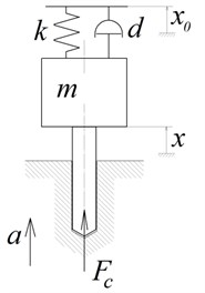
a) General model

b) Cutting zone

2. Model description

The computational scheme of vibratory drilling with kinematic excitation is presented in Fig. 1. The system of equations, in dimensionless form, describing the vibratory head dynamics is presented by Eqs. (2)-(5) [9]:

where: $q=x/a$ – dimensionless axial tool displacement, $q_0=x_0/a$ – dimensionless kinematic excitation, $P_c=F_c/ka$ – dimensionless cutting force, $\eta =h/a$ – dimensionless uncut chip thickness, $\mathrm{\Lambda }=s/a$ – dimensionless axial coordinate of the surface, $\tau =t/T$ – dimensionless time ($T$ – period of a cutting edges pass), $p=\sqrt{k/m}/z\mathrm{\Omega }$ – ratio of eigenfrequency of a vibratory head moving part to the tooth passing frequency ($\mathrm{\Omega }$ – tool rotation rate, $z$ – number of cutting edges), $\zeta =d/2\sqrt{km}$ – dimensionless damping coefficient, $k_c=K_c/k{a}^{1-r}$ – dimensionless cutting coefficient ($K_c$, $r$ – experimental coefficients).

The system of nonlinear Eqs. (1)-(4) includes delayed argument. Solution is calculated numerically, by iterative method, described in [9].

Solution presents the time history of drill displacement and cutting force. To investigate effects of $p$, $k_c$ parameters on vibro-drilling process behavior, the following integral characteristics are introduced: the peak-to-peak displacement, the maximum cutting force and the cutting continuity index. These parameters are described in [9] and calculated after transient process has been finished.

3. Control strategy

Similar to [9], it is assumed that the control law is proportional to velocity of the vibratory head moving part:

where $b$ is the velocity feedback gain.

The strategy of the feedback gain $b$ adaptation by cutting continuity index is proposed in [9]. There it was demonstrated that the closed loop system “self-excited vibratory head – cutting process – control system” shows unstable behavior under certain machining parameters combination. This problem of the proposed control strategy is caused by the fact, that cutting continuity index is not sufficiently sensitive to variations of the system dynamic behavior at stage of vibration arise, when chip segmentation have not yet started.

In the present paper the feedback gain $b$ adaptation is implemented taking into account the peak-to-peak displacement of a vibratory head moving part. It should be mentioned that only peak-to-peak displacement criterion does not allow straight control of chip segmentation process. So, it is desirable to perform adaptation of the coefficient $b$ by using both peak-to-peak displacement and cutting continuity index [9] control.

Remind that computations of the cutting continuity index $\psi$ and the peak-to-peak displacement $A$ are carried out by using equations, presented in [9]:

where ${{\rm T}}_A$ is a dimensionless time interval under consideration. ${{\rm T}}_A=$ 2 is specified for realization of control action. ${{\rm T}}_A=$ 100 is used at the stage of simulation results representation.

Thus, the dependences Eqs. (6), (7) allow computing values of the peak-to-peak displacement $A$ and the cutting continuity index $\psi$ for a discrete set of $\tau$ values. Calculation of $A$ and $\psi$ is carried out using the time step ${{\rm T}}_A$ in the present paper. That is, the set of values ${\tau }_j=j{{\rm T}}_A$, $j=$1, 2,… is introduced, and calculation of $A\left({\tau }_j\right)$ and $\psi \left({\tau }_j\right)$ is carried out by using Eqs. (6), (7) for each $j$.

Further, the two adaptation strategies of the feedback gain $b$ are introduced: the adaptation by peak-to-peak displacement and the mixed adaptation by peak-to-peak displacement with cutting continuity index.

3.1. Strategy of the feedback gain adaptation by peak-to-peak displacement of a vibratory head moving part

The control objective is assuring the required peak-to-peak displacement $A_0$. In case of pure kinematic harmonic excitation of a tool, chip segmentation is ensured if the following condition has been fulfilled [1]:

8

$A\ge \frac{a}{\mathrm{s}\mathrm{i}\mathrm{n}\left(\pi \mathrm{}i\right)},$

where $A$ – peak-to-peak displacement, m; $a$ – tool feed per tooth, m/cutting edge; $i$ – fractional portion of oscillation count, done by an instrument during one cutting edge pass. The relation Eq. (8) proves, that the minimal peak-to-peak displacement $A_0$, required for chip segmentation, is equal to the tool feed per tooth and $i=j-1/2$, $j\in \mathbb{N}$.

It should be mentioned that the peak-to-peak displacement value, assuring chip segmentation, could exceed the tool feed per tooth significantly, in case of not optimal choice of parameter $p$, which effects on the parameter $i$ in Eq. (8).

The algorithm of parameter $b$ adjustment ensuring the required peak-to-peak displacement $A_0$ value is presented below. Fundamental advantage of peak-to-peak displacement $A$ control over cutting continuity index $\psi$ control is the possibility to take into account the dynamic behavior of vibro-drilling process at stage when chip segmentation has not started yet.

Similar to [9] let us propose the linear dependence of parameter $b$ adaptation:

9

$\dot{b}=c\left(A_0-A\right),$

where $c$ is adaptation factor.

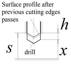
In the parameter $b$ adaptation algorithm, described below, the Eq. (9) is used not for all values of $A$. Let us consider Fig. 2, presenting a Poincare diagram of the tool axial motion. That diagram was constructed as following: a set of simulations were carried out for different values of the parameter $k_c$, extremes of motions were defined for each simulation on second half of the corresponding time history. Those points corresponding to each $k_c$ value are marked in Fig. 2. The model [9] without control was used for those computations.

Fig. 2 shows that vibrations fade out and continuous cutting with the settled uncut chip thickness is registered if parameter $k_c$ is below the certain critical value $k_c^{*}$. When this critical value $k_c^{*}$ has been exceeded, the system behavior changes abruptly. The vibrations are stabilized with peak-to-peak displacement defined by two extremum points on the diagram. Such behavior correlates well with the subcritical bifurcation type [10] when loosing stability due to the regenerative effect.

Consequently, when specifying control excitation, the linear relation Eq. (9) for parameter $b$ derivative is used within the certain interval near the required value of $A$:

10

$A\in \left[g_1{A}_0,g_2{A}_0\right],$

where $g_1$, $g_2$ are prescribed coefficients, $g_1<$1, $g_2>$1. Interval Eq. (10) is marked in Fig. 2 by hatching.

Fig. 2Poincare diagram presenting dependence of displacements extremes from parameter kc at p= 1.5 without control. Hatched region presents the region where the linear equation for parameter b adaptation is chosen

If the peak-to-peak displacement $A$ is out of interval Eq. (10), it’s advisable to speed up achieving a vibration mode with required characteristics. So the use of qualitatively other strategies for parameter $b$ computations is proposed in that case.

It’s necessary to estimate the rate of the peak-to-peak displacement increase at the stage of vibration growth. The following characteristic could be introduced as such estimate:

11

$\tilde{\lambda }=\frac{1}{{{\rm T}}_A}\mathrm{l}\mathrm{n}\frac{A\left(\tau \right)}{A\left(\tau -{{\rm T}}_A\right)}.$

Cutting forces, control excitation and inelastic interactions in the vibratory head all together determine the rate of peak-to-peak displacement growth, calculated by using the Eq. (11). To estimate the control action effect on rate of peak-to-peak displacement growth let us substitute the Eqs. (5) in (1) and assume the value of the cutting force $P_c=$0:

12

$\frac{1}{{\left(2\pi p\right)}^2}\ddot{q}+\left(\frac{\zeta }{\pi p}-b\right)\dot{q}+q=0.$

The value $\tilde{\lambda }\text{,}$ calculated by using Eq. (11) for the solution of Eq. (12), is equal to ${\left(2\pi p\right)}^2\left(b-(\zeta /\pi p)\right)/2$.

Therefore let us introduce the characteristic Eq. (13) to compute rate of peak-to-peak displacement growth due to only cutting forces and inelastic interactions in the vibratory head:

13

$\lambda =\frac{1}{{{\rm T}}_A}\mathrm{l}\mathrm{n}\frac{A\left(\tau \right)}{A\left(\tau -{{\rm T}}_A\right)}-\frac{1}{2}b{\left(2\pi p\right)}^2,$

where $b$ is the velocity feedback gain value within the interval $\tau \in \left[\tau -{{\rm T}}_A,\tau \right)$.

Calculation of $\lambda$ by using Eq. (13), allows to define a new value of the coefficient $b$:

14

$b^{\mathrm{*}}=\frac{1}{{\left(2\pi p\right)}^2}\cdot 2\left(\frac{1}{{\mathrm{{\rm T}}}_D}\mathrm{l}\mathrm{n}\frac{A_0}{A\left(\tau \right)}-\lambda \right),$

where ${{\rm T}}_D$ is desired time of settling down of the vibration mode to the required peak-to-peak displacement. The coefficient $b$ value for implementation on the next time interval $\tau \in \left[\tau ,\tau +{{\rm T}}_A\right)$ is calculated by using the Eq. (14).

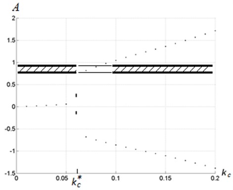
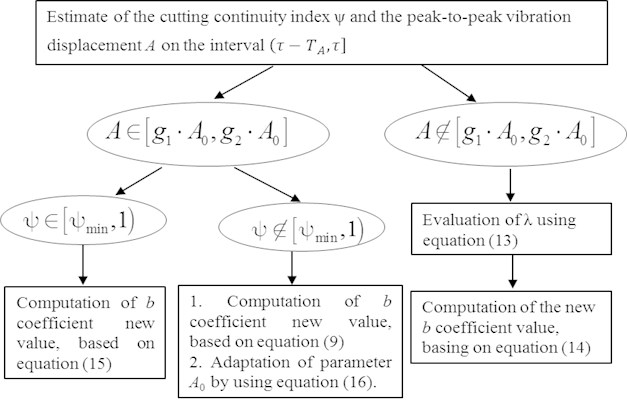
Complete algorithm of the coefficient $b$ adaptation is presented in Fig. 3. Calculation of $b$ coefficient is carried out with time interval ${{\rm T}}_A$.

Fig. 3Algorithm of coefficient b adaptation by peak-to-peak displacement A

3.2. Strategy of the mixed feedback gain adaptation by peak-to-peak vibration displacement and by cutting continuity index

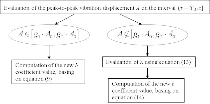
The control objective is ensuring the required value of cutting continuity index ${\psi }_0$. Adaptation algorithm is presented in Fig. 4. The idea (gist) of the control strategy consists of two interconnected parts: the parameter $b$ adaptation by the peak-to-peak displacement $A$ same as in the Section 3.1 and $A$ required value adaptation depending on cutting continuity index $\psi$.

Fig. 4Algorithm of the mixed adaptation of b coefficient by peak-to-peak displacement A and by cutting continuity index ψ

In that adaptation algorithm, the value of peak-to-peak displacement is calculated by using the Eq. (7) and related to the values of $g_1{A}_0$ and $g_2{A}_0$, where: $g_1$, $g_2$ are configurable parameters, $A_0$ is the target value of peak-to-peak displacement $A$. In the case $A\notin \left[g_1{A}_0,g_2{A}_0\right]$, the feedback gain $b$ is calculated by algorithm described in Section 3.1 for such case.

In the case $A\in \left[g_1{A}_0,\mathrm{}{g}_2{A}_0\right]$, computation of cutting continuity index is carried out by using Eq. (6). If chip segmentation occurs and index $\psi$ is not excessively low, that is $\psi \in \left[{\psi }_{\mathrm{m}\mathrm{i}\mathrm{n}},\mathrm{}1\right)$ (${\psi }_{\mathrm{m}\mathrm{i}\mathrm{n}}$ – some prescribed parameter), then correction of the feedback gain is required only to bring $\psi$ nearer to the required value. Calculation of $b$, same as in [9], is carried out by using equation:

15

$\dot{b}=c\left(\psi -{\psi }_0\right).$

In the case $A\in \left[g_1{A}_0,\mathrm{}{g}_2{A}_0\right]$ and there is no chip segmentation observed ($\psi =$1) or cutting continuity index is too low ($\psi <{\psi }_{\mathrm{m}\mathrm{i}\mathrm{n}}$), then target correction of the peak-to-peak displacement is required. In the present paper, the value of peak-to-peak displacement correction is assumed to be proportional to the difference between actual and the target value of index $\psi$:

16

$A_0^{new}=A_0+c_A\left(\psi -{\psi }_0\right),$

where $A_0$ – value of the peak-to-peak displacement specified before correction, $A_0^{new}$ – after correction, $c_A$ – adaptation coefficient, herein $c_A=$1.

It is desirable to carry out the adaptation Eq. (16) of the peak-to-peak displacement target value $A_0$ keeping peak-to-peak displacement value within an interval $\left[g_1{A}_0,\mathrm{}{g}_2{A}_0\right]$. Therefore the adaptation of $A_0$ is performed together with the following adaptation of $b$ coefficient:

17

$\dot{b}=c\left(A_0-A\right).$

Thus, the described algorithm allows to control the rate of the peak-to-peak displacement growth, at the stage when chip segmentation has not been started yet, and allows to apply “fine” adjustment of the feedback gain $b$ assuring the target cutting continuity index.

4. Results of modeling

The results of multi-variant simulation of system dynamics are presented. Two variants of control algorithms, described in Section 3, are considered. Integral processes characteristics are calculated for a set of parameters $p$ and $k_c$ combinations. The following system parameters values were used for simulation: $\zeta =$ 0.01, $r=$ 0.75, $c=$ 0.001, $A_0=$ 1.2, ${\psi }_0=$ 0.9, ${\psi }_{\mathrm{m}\mathrm{i}\mathrm{n}}=$0.5, $g_1=$0.9, $g_2=$1.5, ${{\rm T}}_D=$10. The integration time step is $\mathrm{\Delta }\tau ={\tau }_{j+1}–{\tau }_j=$ 0.01, the dimensionless integration time – 500. Maps of peak-to-peak displacement $A$ and cutting continuity index $\psi$ are presented in the Fig. 5.

The method of maps construction is described in [9]. Dimensionless parameter $p$ is marked along $x$-axis and dimensionless parameter $k_c$ – along $y$-axis. The following four variants of simulation are considered: without control, with control by cutting continuity index (both were described and investigated in [9]), proposed in this work control by the peak-to-peak displacement and mixed control by the peak-to-peak displacement and the cutting continuity index. For brevity sake of the results description, let us denote the above mentioned control strategies as the strategy 1, strategy 2 and strategy 3 respectively. Maps of peak-to-peak displacement for cases without control and with control by strategy 1 (Fig 5 (а), (b), (e), (f)) were obtained and described in [9].

Maps of the peak-to-peak displacement and the cutting continuity index for the case of strategy 2 are presented in Fig. 5(с), 5(g). Fig. 5(с) illustrates that such method of the feedback gain $b$ adaptation allows maintaining a target peak-to-peak displacement in a wide range of machining parameters. Fig. 5(g) illustrates that under such control algorithm the desired value of cutting continuity index $\psi$ (about 0.8-0.9) is reached in the area contoured by the dashed line on the machining parameters plane. Whereas for the case without control such interval is approximately equal to 0.

Maps for case of control strategy 3 are presented in Fig. 5(d), 5(h). Fig. 5(h) shows that in case of such control strategy, the range of machining parameters corresponding to the required vibro-drilling mode is considerably increased when compared with the strategy 2 (Fig. 5(g)). But the region with desirable value of index $\psi$ is still limited because of constraints on control excitation (see [9]).

Thus, when applying the strategies 2 and 3 proposed in this work, chip segmentation with desirable value of the index $\psi$ will be ensured even if essential error (about 30-40 %) exists in the cutting stiffness $k_c$ determination.

There were 5 points on the machining parameters plane (see Fig. 6) considered in detail in [9]: $A$ ($p=$1.5; $k_c=$0.1), $B$ ($p=$1.5; $k_c=$0.02), $C$ ($p=$1.5; $k_c=$0.6), $D$ ($p=$1.7; $k_c=$0.1), $E$ ($p=$1.2; $k_c=$0.1). Remind that for points $B$ and $E$ strategy 1 do not provide control objectives achievement due to the instability of the control algorithm, and for the point $C$ – because of insufficient power of the actuator. Herein the dynamic system behavior under control strategies 2 and 3 is investigated only for two most representative points: $B$ and $D$. In respect of the other 3 points out of 5 mentioned above (Fig. 6) the conclusion is following: at point $A$ strategies 2 and 3 ensures the desired results of the control; at point $C$ the desired results are not achieved; at point $E$ – chip segmentation is ensured only with control strategy 3.

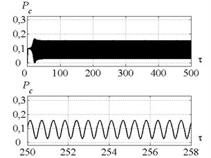
Fig. 7, 8 presents time histories for the point $B$ (Fig. 6) in the case of the control strategies 2 and 3 respectively. Fig. 7 proves that control strategy 2 ensures the peak-to-peak displacement on the target level. Cutting forces regularly reach zero on the diagrams, proving that cutting process is periodically interrupted and chip is segmented. Cutting continuity index is equal to 0.81.

Fig. 5Maps of the steady-state parameters of the oscillating cutting process. Left hand side а), b), с), d) –maps of peak-to-peak vibration displacement A, right hand side e), f), g), h) – maps of cutting continuity index ψ. On the top а), e) – without control; b), f) – control strategy 1; с), g) – control strategy 2; d), h) – control strategy 3

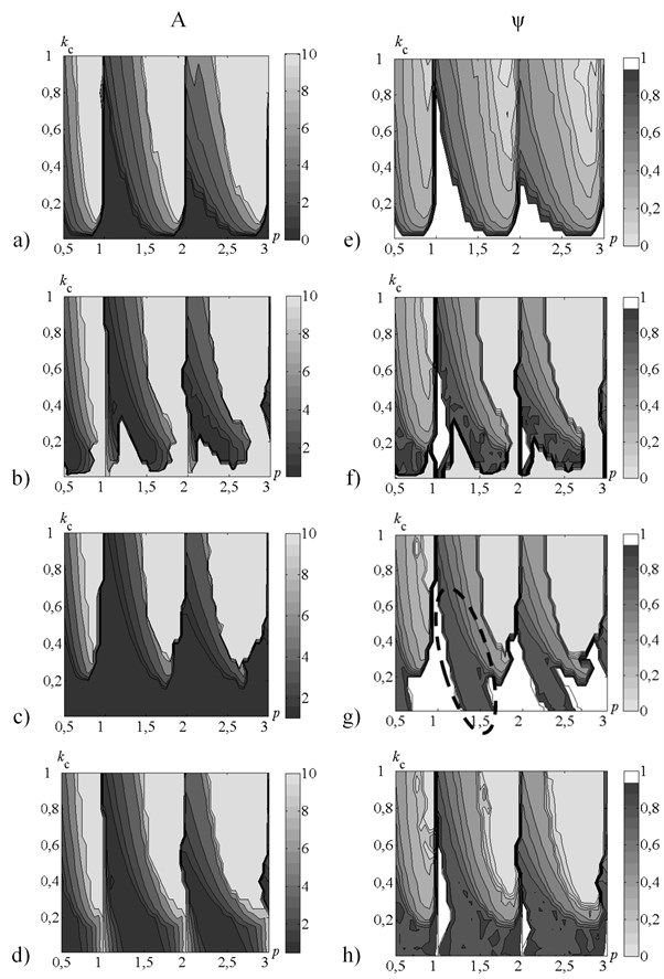
Fig. 6Allocation of points, for which time histories are presented. Points are on the map of cutting continuity index without control. Solid black thick lines represent the stability borders of linearized system

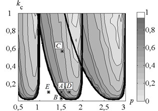
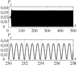
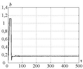
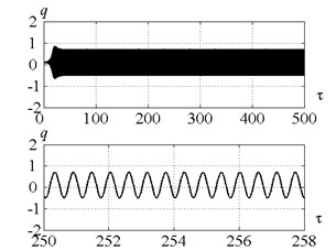
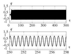
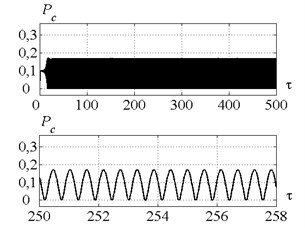
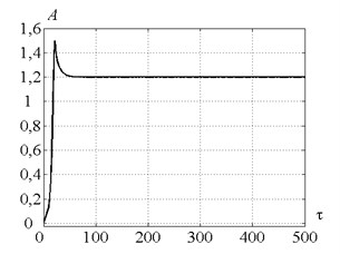
Fig. 8 proves that control strategy 3 ensures the peak-to-peak displacement on the level of less than 1.2, indicating redundancy of the initially specified value of $A_0$. Cutting continuity index is equal to 0.9. Velocity feedback gain reaches its maximum on the first stage of the vibro-drilling process, due to the necessity of energy supply to the system at the stage of vibration arise. Then, coefficient $b$ stabilizes at the constant positive value, indicating continuous energy supply to the dynamic system. This energy flow is needed to overcome the significant dynamic system dissipation, that doesn’t allow self-excited vibrations arise, as shown in [9]. Note, that in the case of the control strategy 2 the peak-to-peak displacement $A$ and the feedback gain $b$ vary in time similar to strategy 3 with the only exception: $A$ is stabilized on a priori specified value 1.2.

Fig. 7a) Time history of a tool motion and b) cutting force in the case of control strategy 2. The values of the parameters p and kc correspond to the point B

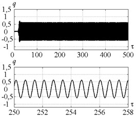
a)

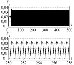
b)

Fig. 8a) Time history of tool motion, b) cutting forces, c) velocity feedback gain and d) peak-to-peak vibration displacement in the case of control strategy 3. The values of the parameters p and kc correspond to the point B

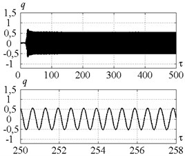
a)

b)

c)

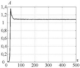
d)

Thus both strategies 2 and 3 ensure chip segmentation in point $B$. But in the point $D$ chip segmentation is obtained only with the control strategy 3.

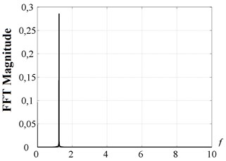
Fig. 9, 10 present time histories for point $D$ (Fig. 6) in case of control strategies 2 and 3 respectively. Fig. 11 presents time history of peak-to-peak displacement at point $D$ (Fig. 6) for the control strategies 2 and 3. Fig. 11(a) indicates that the control strategy 2 ensure the peak-to-peak displacement on the target level. But the cutting force doesn’t achieve zero at the steady-state process stage (see Fig. 9), so chip segmentation doesn’t occur. Fig. 5(g) shows that the peak-to-peak displacement at the level near the target value of 1.2 is ensure for the considerable area on the plane of the parameters $p$, $k_c$. But chip segmentation is ensured only within a small part of that area adjoined to values $p=$ 0.5; 1.5; 2.5…. To explain that fact let us consider the spectrum of the tool displacements at the point $D$, presented in Fig. 12. The ratio of tool vibration frequency to the tooth-passing frequency is drawn along $x$-axis. Fractional part of that value is equal to $i$ in Eq. (8). The spectrum shows that for the point $D$ the parameter $i$ considerably differs from its optimal value ($i=$ 0.5; 1.5; 2.5…, see Introduction). Thus, much higher peak-to-peak displacement values are required to ensure chip segmentation under given conditions. So, the lack of the strategy 2 is caused by the independence of the target value of peak-to-peak displacement on the cutting continuity index.

Fig. 9Time history of a tool motion (on the left) and cutting force (on the right) in the case of control strategy 2. The values of the parameters p and kc correspond to the point D

a)

b)

Fig. 10a) Time history of a tool motion and b) cutting force in the case of control strategy 3. The values of the parameters p and kc correspond to the point D

a)

b)

Fig. 11a) Time history of a tool peak-to-peak vibration displacement in case of control strategy 2 and b) control strategy 3. The values of the parameters p and kc correspond to the point D

a)

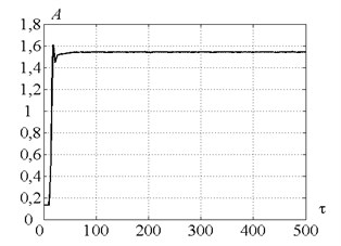
b)

Fig. 12Spectrum of the tool motion for the point D in case of control strategy 2

The strategy 3 takes into account the target value of cutting continuity index ${\psi }_0$ and therefore leads to chip segmentation under the same cutting conditions (point $D$) by means of the target peak-to-peak displacement value adjustment (see algorithm in Fig. 4). Fig. 10 proves that the control strategy 3 ensures chip segmentation. It is evident from the Fig. 11(b) that using of the control strategy 3 leads to peak-to-peak displacement steady-state value higher than initially specified value of 1.2.

5. Conclusions

The present work considers algorithms of vibratory drilling process control with two methods of the feedback gain adaptation: the adaptation by the peak-to-peak displacement (strategy 2) and the mixed adaptation by peak-to-peak displacement with cutting continuity index (strategy 3). In this paper results of the investigation of the closed loop system “self-excited vibratory head – cutting process – control system” behavior is presented.

Mathematical modeling had been carried out for the number of combinations of the rotation rates and the cutting coefficients values. It was proved that proposed control algorithms ensured the reliable chip segmentation at a wide range of machining parameters combinations. It should be noted that the strategy 3 ensures chip segmentation at a wider range of machining parameters combinations than the strategy 2 does, due to the target peak-to-peak displacement value adjustment according to the specified value of cutting continuity index. Chip segmentation with desirable value of the cutting continuity index is ensured even with cutting coefficient uncertainty up to 100 % (e.g. with $p=$1.3 and specified $k_c=$ 0.2) when certain values of the parameter $p$ are chosen.

The implementation of the both proposed strategies ensures quicker stabilizing of the vibration mode than in the case of control by the cutting continuity index only (the strategy 1). That quick stabilizing is possible due to the control by peak-to-peak displacement, which is more sensitive to the system dynamic behavior variations, than the cutting continuity index.

There are considerable areas where amplitudes of the piezo actuator elongations are insufficient for assuring of the intermittent cutting conditions. So in the following works it is desirable to consider other means to provide energy to the vibrating system.