A two-step method composed of wavelet transform and model updating method for multiple damage diagnosis in beams

Abbasnia, Reza; Mirzaei, Borhan; Yousefbeik, Seyedmohamadmahdi

doi:10.21595/jve.2016.16721

Journal of Vibroengineering

Browse Journal

Submit article

Published: 15 May 2016

Check for updates

A two-step method composed of wavelet transform and model updating method for multiple damage diagnosis in beams

Reza Abbasnia¹

Borhan Mirzaei²

Seyedmohamadmahdi Yousefbeik³

^{1, 2}Center of Excellence for Fundamental Studies in Structural Engineering, School of Civil Engineering, Iran University of Science and Technology, P.O. Box 16765-163, Tehran, Iran

³School of Civil Engineering, Iran University of Science and Technology, Tehran, Iran

Corresponding Author:

Borhan Mirzaei

Cite the article Download PDF

Downloads 1416

WoS Core Citations 4

CrossRef Citations 3

Abstract

In the present study, a two-step approach comprised of wavelet transform and model updating method for multiple structural damage localization and quantification in beams is proposed. The first step is commenced with applying wavelet transform to axial components of mode shapes so as to predict where the damages are located. During this step, wavelet transform might mistakenly detect a number of elements as impaired due to both sampling interval and middle support effect. In the next step, by defining a damage sensitive objective function consisting of natural frequencies and mode shapes, damage intensities at predicted locations will be computed via model updating method employing ECBO (Enhanced Colliding Bodies Optimization) algorithm. The problem with mistakenly predicted damaged locations will be addressed by reported damage intensities during the second step. The present study also indicates that this two-step method greatly assists in reducing the number of variables during model updating process leading to more precise results. Three numerical examples with multiple damages and noisy modal data are studied in order to guarantee the efficacy of the method. Moreover, one numerical example is solved with a number of other Meta-Heuristic algorithms including GA (Genetic Algorithm), CSS (Charged System Search), Pattern Search and Cuckoo algorithm whose results are compared to ECBO algorithm with the intention of ensuring the veracity of ECBO results. The results vividly demonstrate that this method is highly efficient even in the presence of noise.

1. Introduction

Due to various loading conditions, structures may undergo some damages which might be either partial or significant. As a result, Structural Health Monitoring (SHM) and Damage Detection methods perform a pivotal role in ascertaining the location and intensity of possible damages. In this respect, researchers and scholars have made a great effort to bring forth new approaches that are able to spot the location of the damage and identify its intensity. Amongst them, it may be referred to Local methods including Acoustic, Ultrasonic, Radiograph, Microwave, Thermal field. Of the Global methods, it could be pointed to Frequency Based, Mode Shape based, Model Updating, and Wavelet Analysis and so on. A comprehensive summary about multifarious methods by which damage could be diagnosed is provided in [1-3].

Wavelet transform has been a robust and apposite method of choice by a number of researchers, which owes its credit to high capability of pinpointing singular points both in signal itself and its derivatives, irrespective of what type of signal it is -either stationary or non-stationary, as opposed to other mathematical transforms [4] such as Fourier. References [5-7] were possibly the first scholars analyzing numerical and experimental deflection in a damaged simply supported beam with wavelet, and also demonstrated that damage will be expressed in a deflection curve in the form of a singular point (in both deflection and its derivatives), and as a result, wavelet transform could be utilized in the process of detecting damage. A comprehensive review of wavelet transform and its applications could be seen in [8].

In the roughly most literature of damage detection methods by wavelet, location and not severity of damages are just diagnosed. An illustration of this is in [9, 10] in which wavelet transform was employed to spot damage in beams, and the same method was used in [11-13] to detect damage in plate structures. Other researchers could be named like [14, 15], who assisted to develop the capability of wavelet transform to pinpoint damages. In reference [16] mode shape curvature modification and denoising are studied to enhance the resolution of wavelet, and it was benefitted from a complex mother wavelet in Euler Beams in [17] in order to spot multiple cracks more precisely.

However, in a handful of references, some indirect and statistical methods are proposed to identify damage severity by wavelet transform. An indication of this would be seen in [10, 13, 18, 19] in which the intensity of damage is estimated by a linear regression between the maximum value of wavelet coefficient and related damage intensity. In this regard, apart from statistical methods, a number of two-step methods have been proposed, which have received more attention among scholars. An indication of this is in [20] which propounds an automated procedure based on wavelet and meta – optimization process for fault diagnosis in sandwich structures. In [21] a damage detection method comprised of wavelet analysis and Artificial Neural Network (ANN) with respect to modal response is offered, which applies wavelet transform on vibrational responses to spot the position of damages while ANN was employed to find out damage intensities. A two-step technique is discussed in [22] recruiting EMD (Empirical Mode Decomposition) to decompose the modal response to its mono-component signals and then, the characteristics of damages will be identified by exerting wavelet on that mono-component signals. Another example of two-step method would be observed in [23] through which two dimensional wavelet is applied on a plate mode shape to disclose the position of damages and then, PSO algorithm was utilized to quantify the severity of damages.

In the present study, two-step method composed of wavelet approach and model updating via ECBO algorithm is propounded so as to reveal the intensity of damages as well as locating them. In the first step, wavelet transform will be applied on axial mode shape in order that the location of damages would be nominated. During this step, a handful of regions would mistakenly emerge as damaged in wavelet coefficient; however, this issue will be tackled in the second step where an objective function is presented based on which the intensities will be computed via ECBO algorithm and model updating.

2. Background

2.1. Step 1: Locating damaged elements

2.1.1. Continuous wavelet transform (CWT)

Owing to multi – resolution properties of wavelet transform, wavelet is able to perform as a magnifying glass of signal which could closely scrutinize both stationary and non-stationary signals more precisely in order to reveal details of signal, which is one of its merits in comparison with other traditional signal processing tools. Below, a concise introduction to mathematical definition of wavelet transform is provided. The mathematical definition of wavelet transform was first defined in [24] as below:

1

C W T_{C o e f f} = W_{f} (a, b) = \frac{1}{\sqrt{a}} \int_{- \infty}^{+ \infty} f (x) \bar{ψ} (\frac{x - b}{a}) d x .

In above, $ψ (x)$ is a mother wavelet function with zero mean value for which satisfying two essential conditions is imperative [25]. In above equation $a >$ 0 and $a$ , $b$ are both real. The variable “ $a$ ” represents mother wavelet width (scale), which stretches or shrinks mother wavelet, and variable “ $b$ ” represents the translation along length axis. $\bar{ψ} (x)$ is the conjugate complex of $ψ (x)$ , $W f (a, b)$ are wavelet coefficients of $f (x)$ .

The crucial and striking point which should be taken into account is that spotting damaged regions via wavelet transform is viable with different displacement components (translational – rotational – axial) either in statically or free vibration analysis. Different components of displacement in free vibration of a beam are schematically shown in Fig. 1 and Eq. (5). Both translational components and rotational ones have been used by wavelet transformation [26] while damage detection by axial components and wavelet had not been used for beams before, and in the present study its usability for damage detection and sensitivity to noise will be verified. It should be noted that longitudinal free vibration mode shape was used for rods to detect damage location by wavelet [26] as well as in walls by Curvelet transform [27].

In a group of references, wavelet transform is applied on the subtraction between characteristics of the intact structure and the damaged one [28-31] and [16], which, in turn, sheds more light on damage location. Similarly, in this paper, the process of damage detection is applied on subtraction of axial components for intact and damaged beam, whose results are compared to translational and rotational components to evaluate its usability. More numerical examples will be given in the following sections:

2

Frequency analysis \overset{results}{\to} mode shape matrix,

[f_{i j}] = [{\{f\}}_{1}, {\{f\}}_{2}, \dots, {\{f\}}_{n}],

{\{f\}}_{i} = {\underset{n c o m p o n e n t}{\underset{⏟}{[r_{1}, r_{2}, \dots, v_{1}, v_{2}, \dots, a_{1}, a_{2}, \dots]}}}^{T},

where $[f_{i j}]$ is mode shape matrix, $n$ number of mode shape and degree of freedom, $r$ is rotational, $v$ is vertical or translation, $a$ is axial components.

Fig. 1First mode shape of a clamped – simple beam

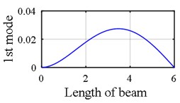
a) Translational components

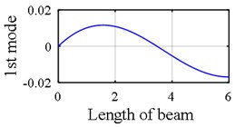
b) Rotational components

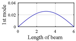
c) Axial components

2.1.2. Edge effect (outer support effect)

Aside from damaged area, another area might appear as damaged in wavelet coefficients which would be attributed to signal border points which is resulted from the fact that wavelet transform is an integration from minus infinity to plus infinity while deflection curve or signal length is defined through a finite length. This problem, which is called edge effect or border distortion, would be simply tackled by extending the signal virtually. New and traditional approaches of omitting border distortion is reviewed and discussed in [16, 32].

2.1.3. Middle support effect (inner support effect)

Another issue for pinpointing damage location is middle support effect. There are, indeed, other locations emerging in the deflection curve as singular (damage) whereas they are intact. Interestingly, an illustration of this would be observed in free vibration of two span beams in axial mode shapes (Fig. 9-11, Fig. 14, Fig. 15) during which the middle support will appear as damaged in wavelet coefficient since in each mode, the left hand slope and the right hand one are not identical at middle support, so it will cause fluctuation in wavelet coefficient.

Despite the fact that applying signal extension methods [33] is able to exclude the edge effects effectively, it is not efficient to deal with middle support effect. Using modal updating via optimization algorithms in the second step of the present article, presuppose that these points (middle elements) are hypothetically damaged, yet it will be clarified that damage intensities in these points are zero. Thus, by this innovative method the middle support effect will be tackled (Section 3.2.2 and 3.2.3).

2.1.4. Sampling interval effect

One of the most important factors aiding in detecting damage location with wavelet transform is sampling interval or structural elements size. Damage detection with wavelets is heavily reliant upon the size of elements (sampling intervals) as well as size of damage in a way that if the number of elements along the beam are inadequate, the possible damage might be overlooked. Similarly, in case that damage is very small, it might remain masked during damage prognosis process. In [33, 34, 35] this problem is discussed.

In order that sampling interval effect would be observed, a simply supported beam with 3 damages (0.8-1, 2-2.2, 3-3.2) is modeled with two different sampling intervals, one of which has 125 elements and the other one is modeled with 25 elements, and as is clearly presented in Fig. 2, the resolution of model with 125 elements is far more than the other one. But in this paper, this drawback is reciprocated by using model updating via ECBO algorithm mainly because a handful of peripheral elements to damaged area might mistakenly be presumed to be impaired, yet damage intensities resulted from model updating via ECBO algorithm divulge whether or not suspected elements were damaged.

Fig. 2Damage detection in a simply supported beam. Effect of sampling interval could be vividly observed due to different element size

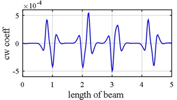
a) 125 elements

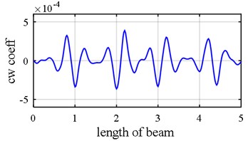
b) 25 elements

2.2. Step 2: Quantifying the intensity of damage

2.2.1. Objective function

So as to propose an efficacious damage detection method based on model updating, which could be both in accord with a variety of optimization algorithms and capable of determining various damages, an appropriate and efficient objective function is requisite. The efficacious objective function ought to be not only inclusive of structural parameters sensitive to impairment even to negligible damage but also insensitive to other parameters like noise.

The initial step to generate an effectual objective function is that the following equation should be satisfied:

3

([K_{d}] - (λ_{j}^{d}) [M]) \{Φ_{j}^{d}\} = 0, j = 1, \dots, n .

In this equation, $[K_{d}]$ and $[M]$ are representative of Global stiffness matrix and Global mass matrix in damaged condition, respectively; $λ_{j}^{d}$ and $Ø_{j}$ delineate square of $j$ th natural frequency and mode shape, respectively, corresponding to $j$ th mode of damaged structure. Number of natural modes is regarded as “ $n$ ”. It should be noted that during damage process, mass is considered immutable:

4

[M] \approx [M_{d}] .

Stiffness reduction is formulated in following equation. Reduction factor $d_{e}$ is a scalar variable varying between 0 and 1 in which 0 means no damage and 1 means completely wrecked:

5

[K_{d}^{e}] = [K^{e}] (1 - d_{e}) .

In Eq. (5), $[K_{d}^{e}]$ and $[K^{e}]$ are local matrices or element matrices related to damaged element and undamaged ones respectively.

Desired objective function is defined as below:

6

F_{o b j} = 1 - M T M A C .

In which:

7

M T M A C = \prod_{j = 1}^{N_{m}} M T M A C_{j},

8

M T M A C_{j} = \frac{F' (\{Φ_{n u m j}\}, \{Φ_{e x p j}\})}{{(1 + {(\frac{ω_{e x p j}^{2} - ω_{n u m j}^{2}}{ω_{e x p j}^{2} + ω_{n u m j}^{2}})}^{2})}^{2}},

9

F_{j}^{'} = \frac{2 * (|{\{x_{j}\}}^{T} \{x_{j}^{*}\}|)}{({\{x_{j}\}}^{T} \{x_{j}\}) + ({\{x_{j}^{*}\}}^{T} \{x_{j}^{*}\})} .

2.2.2. ECBO algorithm

CBO algorithm is a sort of Meta-Heuristic algorithms elevated by Kaveh and Mahdavi [36] and resulted from collision physical laws. Each solution candidate $X_{i}$ , which consists of abundance of variable, is considered as a colliding body. The bodies bifurcate to two distinct groups, moving bodies and inert ones (Fig. 3). The moving bodies follow inert ones till a collision occurs between them. Due to this impact, firstly, the position of moving bodies will be modified, and secondly, it pushes inert bodies to better locations. Aftermath of collision, both velocity and position of colliding bodies will be reconsidered and updated with regard to collision laws.

ECBO (Enhanced colliding bodies optimizations) is, in fact, ameliorated version of CBO with the intent of augmenting fastness and heightening accuracy of algorithm. In other words, it utilizes a memory to keep the optimum CBs and also employs a technique to escape from local minima [37].

Fig. 3The moving bodies a) before the collision b) after the collision [38]

a)

b)

Steps of ECBO algorithm could be succinctly observed as below:

Step 1: the position of each CB would be randomly opted in $m$ dimensional space:

10

x_{i}^{0} = x_{m i n} + r a n d o m_{} (x_{m a x} - x_{m i n}), i = 1, 2, \dots, n .

In which $x_{i}^{0}$ is initial solution vector for $C B_{i}$ and $x_{m i n}$ , $x_{m a x}$ are boundaries for design variables. “rand” is a random vector between [0, 1].

Step 2: each CB’s mass is calculated according to following equation:

11

m_{k} = \frac{\frac{1}{f i t (k)}}{\frac{1}{\sum_{i = 1}^{n} \frac{1}{f i t (i)}}}, k = 1, 2, \dots, n .

Step 3: the best CBs’ vector, mass, value of objective function will be stored in CM (Colliding Memory), then they will be added to population and equal number words CBs will be omitted [38, 39]. Finally, CBs will be sorted in ascending order (Fig. 4(a)).

Fig. 4a) CBs sorted in increasing order b) Colliding bodies pair [38]

a)

b)

Step 4: CBs will be divided into two separate groups namely inert and moving (Fig. 4(b)).

Step 5: velocity of moving masses and inert ones for the situation prior to collision will be computed by:

12

v_{i} = 0, i = 1, 2, \dots, \frac{n}{2},

13

v_{i} = x_{i - \frac{n}{2}} - x_{i}, i = \frac{n}{2} + 1, \frac{n}{2} + 2, \dots, n .

Step 6: velocity of moving masses and inert ones for the situation subsequent to collision will be computed by:

14

{v'}_{i} = \frac{(m_{i + \frac{n}{2}} + ε m_{i + \frac{n}{2}}) v_{i + \frac{n}{2}}}{m_{i} + m_{i + \frac{n}{2}}}, i = 1, 2, \dots, \frac{n}{2},

15

{v'}_{i} = \frac{(m_{i} - ε m_{i - \frac{n}{2}}) v_{i}}{m_{i} + m_{i - \frac{n}{2}}}, i = \frac{n}{2} + 1, \frac{n}{2} + 2, \dots, n,

16

ε = 1 - \frac{i t e r}{i t e r_{m a x}} .

Step 7: the new position of CBs will be calculated by following equations:

17

x_{i}^{n e w} = x_{i} + r a n d v_{i}^{'}, i = 1, 2, \dots, \frac{n}{2},

18

x_{i}^{n e w} = x_{i - \frac{n}{2}} + r a n d v_{i}^{'}, i = \frac{n}{2} + 1, \frac{n}{2} + 2, \dots, n .

Step 8: a parameter like “Pro” is introduced between (0, 1) and it will be determined that whether any component of CBs would be changed or not. For every CB, Pro will be compared with $r n_{i}$ ( $i =$ 1, 2,..., $n$ ) which is between (0, 1). If $r n_{i} < P r o$ , one-dimension form $C B_{i}$ will be chosen randomly and its value will be regenerated as below:

19

x_{i j} = x_{j, m i n} + r a n d o m (x_{j, m a x} - x_{j, m i n}) .

Step 9: checking the condition of whether or not algorithms would be stopped.

3. Illustrative and numerical examples

3.1. Finite element modeling and wavelet characteristics

The main objective of this paper is to propose a two-step technique based on which both location and intensity of damage would be identified at shorter time and higher accuracy level. Proposed strategy firstly initiates with estimating location of probable damages with wavelet transform. At this step, a number of elements might be erroneously deemed as damaged such as middle support or peripheral area of a damage location owing to reduction of wavelet coefficient resolution (part 2.5). In the next step, damage intensities for suspected areas will be computed via model updating and ECBO optimization algorithm. The chief merit for the second step is for those areas that are mistakenly supposed to be damaged in former stage because the damage intensity of zero would be indicative of the fact that former assumption was wrong, in this way the problem with middle support effect and wavelet coefficients’ resolution will be tackled. Another initiative in this paper is damage diagnosis via wavelet and axial components of mode shape in beam structures. This point has never been dealt with in other references, yet longitudinal components were used for rod structures [26]. It should be noted that the entire procedure (identifying location and intensity) could be done just by using model updating via optimization algorithms(alone), yet on the condition that model updating would be used only, instead of using a two-step approach, the number of variables would grow greatly leading to declining the accuracy and convergence rate. But if wavelet transform is utilized to predict where damages are situated at first, number of variables would reduce significantly for model updating process which in turn, contributes to the fact that optimizer algorithm works faster with more precision.

Three models each of which has different scenarios are employed to pinpoint multiple damages. Density is $ρ =$ 2500 kg/m³, modulus of elasticity is $E =$ 3e10 N/m², and Poisson’s ratio equals to 0.3, cross section of beam is rectangular shape with height of 50 cm and width of 40 cm. Beam model was constructed in ABAQUS using two-dimensional elements (B21) and modal data were achieved by the frequency analysis. Mode shape components and natural frequencies are extracted from ABAQUS at first in order to be used through two-step method. Then, the following steps are applied on them. Firstly, by interpolation technique of order 3 [16], number of points was extended to 256. This process, as illustrated in reference [16], will lead to least possible noise resulted from data acquisition. The process continues with signal extension which cancels out edge effects. The process is followed by subtraction of components of intact and damaged beam (Eq. (21)). Noises are added to characteristics of damaged beam (natural frequencies and mode shapes) and its formula is depicted in Eq. (22). It should be noted that in order to evaluate proposed method more precisely, two kinds of noise level are considered one of which will be added to mode shape ( $η_{1}$ ) and another one will be added to natural frequencies ( $η_{2}$ ). Input data for CWT:

20

\{\begin{array}{l} Δ ϕ_{v, j} = ϕ_{v, j}^{u} - ϕ_{v, j}^{d}, \\ Δ ϕ_{r, j} = ϕ_{r, j}^{u} - ϕ_{r, j}^{d}, \\ Δ ϕ_{a, j} = ϕ_{a, j}^{u} - ϕ_{a, j}^{d}, \end{array}

21

(ϕ^{d})_{n o i s y} = ϕ^{d} (1 + η_{1} ε), (ω^{d})_{n o i s y} = ω^{d} (1 + η_{2} ε),

where $j$ is mode number, $v$ is vertical or translational, $r$ is rotational, $a$ is axial, $η$ is noise level, $ε$ is random value between (0, 1), $ω$ is natural frequency, $ϕ$ is mode shape.

$Ø_{v} =$ Interpolated and extended translational components of mode shape.

$Ø_{r} =$ Interpolated and extended rotational components of mode shape.

$Ø_{a} =$ Interpolated and extended axial components of mode shape.

Subsequently, continuous wavelet transform (cwt) is applied on differences between components of the intact and the damaged beam. Mother wavelet coif2 with 4 vanishing moments and scale 8 is used for desirable performance [34].

3.2. Numerical examples

3.2.1. Simple-clamped beam

Table 1 delineates two different damage scenarios. The first scenario is noise free while in the second scenario, mode shapes of damaged beam are disturbed by 0.5 % noise ( $η_{1} =$ 0.5 %) and natural frequencies are contaminated by 5 % noise ( $η_{2} =$ 5 %). The method through which the noises are exerted in mode shape data and natural frequencies was explicated in former section. The beam is schematically depicted in Fig. 5. The possible regions of multiple damages in simple – clamped beam are firstly revealed by the applying wavelet transform on different mode shape components (Fig. 6(a)-(c)), and then, unmasked damaged areas will be used in the next step. As is vividly observed in Fig. 6(c) axial components identify the location of damages as well as translational and rotational components in noise free scenario.

Table 1Model 1 damage scenarios with aggregate 30 element

Damage pattern 1			Damage pattern 2 ( $η_{1} =$ 0.5 %, $η_{2} =$ 5 %)
Location (m)	Element	Damage intensity (%)	Location(m)	Element	Damage intensity (%)
1.4-1.6	8	10	1.8-2	10	10
4-4.2	21	15	3.2-3.4	17	15
			4.4-4.6	23	20

Fig. 5Model 1 composed of 30 elements

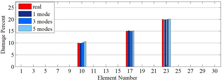
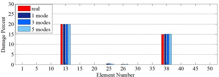
In the next step, the intensity of damages for those nominated areas will be calculated by model updating via ECBO algorithm with 1000 iterations (Fig. 6(d)). In this process, the ECBO algorithm only scrutinizes those nominated areas suspected to be damaged. This procedure greatly enhances the precision of the algorithm and significantly diminishes the number of variables. As is clearly shown in (Fig. 6(b)), the ECBO algorithm reports the intensity of damages as much as they are in table.1 for 1, 3 and 5 modes.

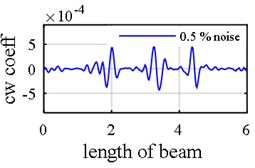
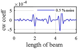
In the following example $η_{1} =$ 0.5 % and $η_{2} =$ 5 % noise are added to mode shape and natural frequency respectively. The main purpose of making data noisy is first to assess that which of three mode shapes components are able to successfully divulge where the damages are located in the presence of noise. As is vividly observed in Fig. 7, both rotational (Fig. 7(a)) and axial components (Fig. 7(c)) are capable of handling 0.5% noise level in mode shape; however, 0.5 % noise added on the translational components (Fig. 7(b)) leads to masking the areas where damages are situated. In addition to that, reporting impeccable results with noisy modal data is illustrative of the fact that proposed objective function is both able to deal with noisy data and sensitive to damage. As it is presented in Fig. 7(d), even in the presence of noise both in mode shape and natural frequency, proposed two-step method accurately revealed not only where the damages are positioned but also how much damage intensities are.

Fig. 6Damage detection in model 1, simple – clamped beam, scenarios 1 (noise free): a) second mode rotational components, b) second mode vertical components, c) first mode axial components, d) damage intensities reported for 1, 3 and 5 modes

Damage detection in model 1, simple – clamped beam, scenarios 1 (noise free): a) second mode rotational components, b) second mode vertical components, c) first mode axial components, d) damage intensities reported for 1, 3 and 5 modes

a)

b)

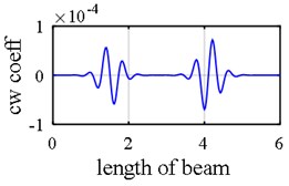
c)

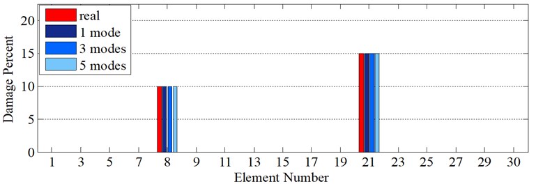
d)

Fig. 7Damage detection in model 1, simple – clamped beam, scenario 2 (η1= 0.5 %, η2= 5 %): a) fourth mode rotational components, b) first mode vertical components, c) third mode axial components, d) damage intensities reported for 1, 3 and 5 modes

Damage detection in model 1, simple – clamped beam, scenario 2 (η1= 0.5 %, η2= 5 %): a) fourth mode rotational components, b) first mode vertical components, c) third mode axial components, d) damage intensities reported for 1, 3 and 5 modes

a)

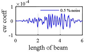
b)

c)

d)

3.2.2. Two-span beam with simple supports

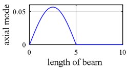
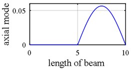
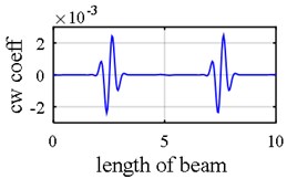
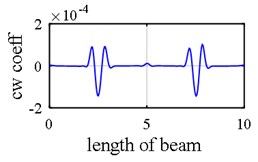
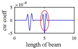
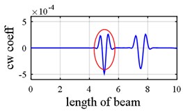
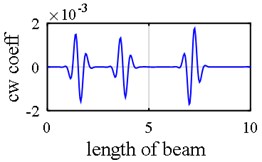
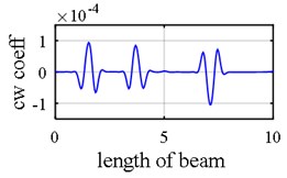
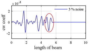
As it was demonstrated in Section 2.1.3, owing to internal support (Fig. 8), a number of singular points might be generated in the axial mode shape that are deemed as damage erroneously during first step because the slope in left hand and right hand sides of the middle support are not identical as is shown in Fig. 9(a), Fig. 9(b), Fig. 10(a) and Fig. 10(b). Consequently, this point (middle support) is unintentionally supposed to be damaged when wavelet transform is applied to axial components (Vividly shown in Fig. 9(e), Fig. 9(f), Fig. 10(e) and Fig. 10(f).

It is better to be noted that “edge effect” or outer supports problem will be effectively annulled by means of signal extension methods; however, signal extension method is not efficacious for middle support effect since middle support is positioned at the inner area of the beam. The second step of the two-step method is the solution to tackle this problem; that is, damage intensity of zero for those mistakenly assumed damaged areas will proof that these elements are intact (Fig. 9(g), Fig. 10(g)). In Table 2, two damage patterns are considered to exemplify this problem.

Fig. 8Model 2 composed of 50 elements

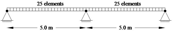
Fig. 9Damage detection in model 2, scenarios 1 (noise free): a) axial 1st mode shape of 2 span beam – left span is active, b) axial 2nd mode shape of 2 span beam – right span is active, c) second mode rotational components, d) third mode vertical components, e) first mode axial components, f) second mode axial components, g) damage intensities reported for 1, 3 and 5 modes

Damage detection in model 2, scenarios 1 (noise free): a) axial 1st mode shape of 2 span beam – left span is active, b) axial 2nd mode shape of 2 span beam – right span is active, c) second mode rotational components, d) third mode vertical components, e) first mode axial components, f) second mode axial components, g) damage intensities reported for 1, 3 and 5 modes

a)

b)

c)

d)

e)

f)

g)

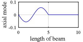
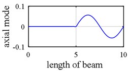
Another phenomenon that occurs in vibration of a two span beam, which would be observed in Fig. 9(a), Fig. 9(b), Fig. 10(a) and Fig. 10(b), is that in each oscillatory mode, half part of a beam is active while the other part is passive-its deformation is equal to zero – which is caused by middle support. That one half of the beam is active in one mode while the other one is inactive, is actually where the “middle support effect” arises from, due to the fact that it leads to inequality of the left hand slope and the right one. Interestingly, this fact also shows that in each mode, the only detectable damaged points are those points which are extant on the active part, so the damage detection process should be made up of observing two mode shapes simultaneously in each of which one part is active and the other is passive. In the Fig. 10(e) and Fig. 10(f) middle support effect is depicted.

Table 2Model 2 damage scenarios with aggregate 50 element

Damage pattern 1			Damage pattern 2			Damage pattern 3 ( $η_{1} =$ 3 %, $η_{2} =$ 5 %)
Location (m)	Element	Damage intensity (%)	Location (m)	Element	Damage intensity (%)	Location (m) element	Damage intensity (%)
2.4-2.6	13	20	1.4-1.6	8	5	The same as damage pattern 2	20
7.4-7.6	38	15	3.6-3.8	19	10		10
			7-7.2	36	15		30

Fig. 10Damage detection in model 2, scenarios 2: a) axial 3st mode shape of 2 span beam – left span is active, b) axial 4st mode shape of 2 span beam – right span is active, c) first mode rotational components, d) first mode vertical components, e) third mode axial components, f) fourth mode axial components, g) damage intensities reported for 1, 3 and 5 modes

Damage detection in model 2, scenarios 2: a) axial 3st mode shape of 2 span beam – left span is active, b) axial 4st mode shape of 2 span beam – right span is active, c) first mode rotational components, d) first mode vertical components, e) third mode axial components, f) fourth mode axial components, g) damage intensities reported for 1, 3 and 5 modes

a)

b)

c)

d)

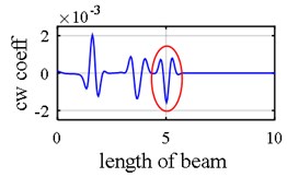
e)

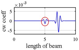
f)

g)

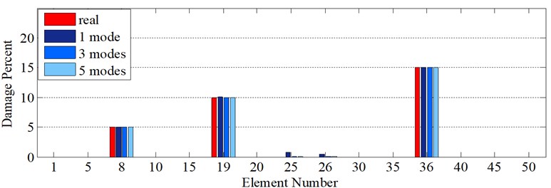
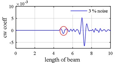
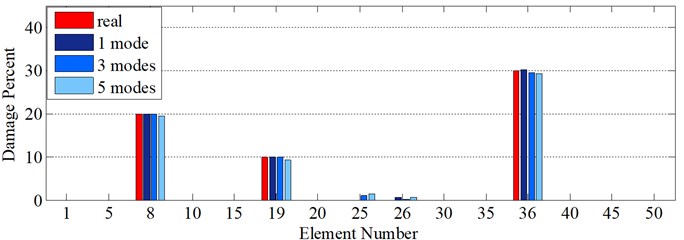
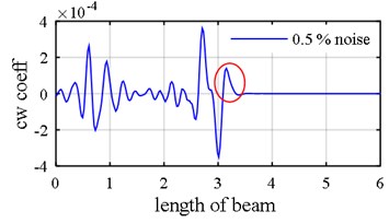
In the following example 3 % noise is added to mode shape ( $η_{1} =$ 3 %) and 5 % noise to natural frequencies ( $η_{2} =$ 5 %). As it was allegorized in the former section and could be observed in Fig. 11(b), translational components of mode shape are much more sensitive to additive noise in comparison with both rotational and axial ones, and it is not capable of exhibiting the location of damages well in the presence of noise. Thus, according to Fig. 11(a), Fig. 11(c) and Fig. 11(d), it is recommended that either rotational or axial components of mode shape data would be used in order to unmask where the damages are positioned in the presence of noise. In Fig. 11(e), it is lucid that not only are the exact damaged elements identified but the intensity of those are also accurately computed when both mode shape and natural frequencies are noisy. The accuracy of damage intensities even in the presence of noise would be attributable to two characteristics. First and foremost, it is not necessary for the optimization algorithm to probe the entire length of the beam, but rather, it just scrutinizes the areas nominated by wavelet transform as damaged. The second characteristic is pertinent to new introduced objective function which is heavily reliant upon damages while not affected by noise. Both of these characteristics considerably assist in diminishing the time of convergence and also to ameliorate the results.

Fig. 11Damage detection in model 2, scenarios 2 (η1= 3 %, η2= 5 %): a) first mode rotational components, b) first mode vertical components, c) third mode axial components, d) fourth mode axial components, b: damage intensities reported for 1, 3 and 5 modes

Damage detection in model 2, scenarios 2 (η1= 3 %, η2= 5 %): a) first mode rotational components, b) first mode vertical components, c) third mode axial components, d) fourth mode axial components, b: damage intensities reported for 1, 3 and 5 modes

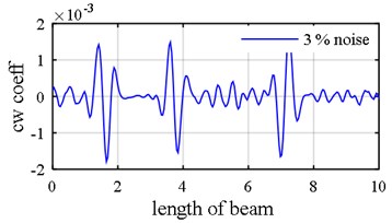
a)

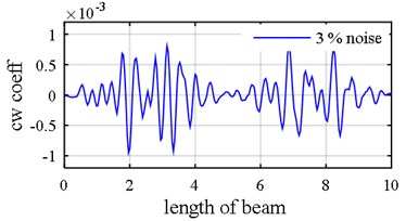
b)

c)

d)

e)

It is worth to mention that as the number of used modes increases, the accuracy of results would diminish when data are contaminated with additive noise stemming from the fact that number of noisy data has grown which is vividly observable in Fig. 11(e). In order that a cyclic method would be classified as reliable and robust, a number of characteristics should be observed. The first and foremost property is attributable to being stable during the whole process which means that the method should exhibit a smooth convergence curve. As it is lucid in Fig. 12, the second step of the two-step method exhibits a smooth cyclic behavior till it converges to desirable answers. Interestingly, with respect to value of the cost function, the fact that results using 1 mode would be better than that of 3 modes, and results for 3 modes would be better than that of 5 modes, can be observed in the iteration curve when noisy data are recruited.

Table 3 reports damage percentages for suspected elements in model 2, scenario2 with $η_{1} =$ 3 %, $η_{2} =$ 5 %. According to this table, in the first 50 iterations, convergence rate is the highest; however, from then onwards convergence rate experiences downward trend and it can be deduced that after the first 500 iterations, the answers do not alter considerably.

Fig. 12Iteration curve for model 2, scenarios 2 with 3 % noise in mode shape and 5 % noise in natural frequency

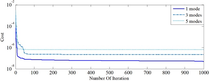
Table 3Damaged intensities captured for suspected elements for model 2, scenarios 2

Number of iterations	Suspected elements
Number of iterations	8	19	25	26	36
2	18.64	19.13	9.89	0.81	36.74
10	18.83	11.96	1.38	0.09	28.91
50	19.15	10.58	1.84	0	29.30
200	19.77	9.87	1.01	0.16	29.58
500	19.84	9.86	0.01	1.14	29.56
1000	20.04	9.88	0	0.52	30.14

3.2.3. Two-span beam with clamped supports - comparison between optimization algorithms

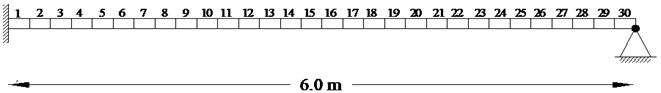
In the following model, a two span beam with two damage scenarios (Table 4) and clamped connection at borders and simple support in its middle is considered (Fig. 13). Sampling interval in this model is 30 cm. As it is clearly shown in Fig. 14, in the first scenario, wavelet transform is exerted only on axial mode shape components with 1 % noise, and then, approximate locations of damages are revealed. Five optimization algorithms scan these areas in order that the intensity of damages would be illuminated. All of them in the presence of 1 % noise in mode shape and 5 % noise in natural frequencies, report the intensity of damages with acceptable accuracy, yet the ECBO algorithm possesses the minimum deviation from real damage value, so it will be concluded that it is more in accord with this two-step procedure (Fig. 14(c)).

Fig. 13Model 3 composed of 20 elements

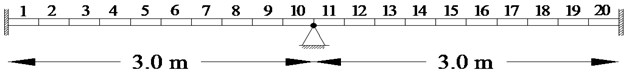
Table 4Model 3 damage scenarios with aggregate 20 element

Damage pattern 1 ( $η_{1} =$ 1 %, $η_{2} =$ 5 %)			Damage pattern 2 ( $η_{1} =$ 0.5 %, $η_{2} =$ 10 %)
Location (m)	Element	Damage intensity (%)	Location (m)	Element	Damage intensity (%)
0.9-1.2	4	15	0.6-0.9	3	10
3.9-4.2	14	15	2.7-3	10	30
			4.2-4.5	15	5
			5.1-5.4	18	20

Fig. 14Damage detection in model 3, scenarios 1 (η1= 1 %, η2= 5 %): a) seventh mode axial components, b) eighth mode axial components, c) damage intensities reported by five Meta-Heuristic algorithms

Damage detection in model 3, scenarios 1 (η1= 1 %, η2= 5 %): a) seventh mode axial components, b) eighth mode axial components, c) damage intensities reported by five Meta-Heuristic algorithms

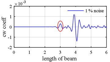
a)

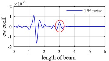
b)

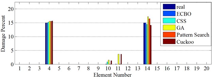
c)

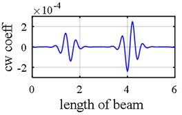
Fig. 15Damage detection in model 3, scenario 2 (η1= 0.5 %, η2= 10 %): a) Third mode axial components (middle support effect is negligible), b) Fourth mode axial components (middle support effect is subordinated due to its nearby damage), c) damage intensities reported by five Meta-Heuristic algorithms

Damage detection in model 3, scenario 2 (η1= 0.5 %, η2= 10 %): a) Third mode axial components (middle support effect is negligible), b) Fourth mode axial components (middle support effect is subordinated due to its nearby damage), c) damage intensities reported by five Meta-Heuristic algorithms

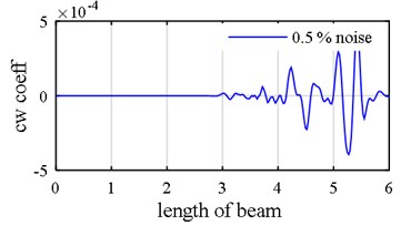
a)

b)

c)

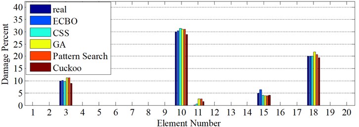
In the second scenario (damage pattern 2), the level of noise in mode shape was halved to 0.5 % while it is heightened for natural frequencies to 1s0 % and also one of the damages is deliberately placed near the middle support (element 10) to assess the fact that whether or not the two-step method is able to detect damage positioned next to middle support in the presence of both noise and middle support effect. This assessment is assumed because the middle support effect, as is depicted in Fig. 15(b), is influenced by the damage fluctuation. Interestingly, all the optimization algorithms identify the element 10 (adjacent to middle support) as damaged with difference that ECBO algorithm shows more precise results (Fig. 15(c)).

4. Conclusions

The present study offers a new two-step method for damage detection of structures with wavelet transform and model updating method. The process is initiated with applying wavelet transform to axial components to identify where the damages took place. The second step continues with exerting optimization algorithms in forms of model updating to unmask the intensity of dubious points. To recapitulate succinctly, following results could be summed up about the two-step method:

1) This two-step method appoints the role of finding damage locations to wavelet transform as well as assigning the responsibility of identifying damage intensities to model updating method.

2) The process of spotting location of damages is verified by applying wavelet transform on the axial components in beam structures. Moreover, its sensitivity to noisy data was evaluated.

3) A new phenomenon called “middle support effect” is both explicated and shown how to tackle.

4) The problem with reduction of wavelet resolution due to “sampling intervals effect” is tackled.

5) Due to employing this two-step method, the number of variables will drastically diminish during model updating process, which, in turn, will result in reducing the process time and augmenting the accuracy of results.

6) An efficient objective function, which uses natural frequencies and related mode shapes, is proposed. Interestingly, it is heavily sensitive to damage while being insensitive to noise. Thus, this objective function is highly recommendable and apposite for damage detection purposes.

7) Five optimization algorithms including GA, Pattern Search, CSS, ECBO and Cuckoo are compared to one another with the the intent of finding the fact that which of them is more compatible with two-step method, and according to the results ECBO algorithm is more in accord with proposed method.

8) To simulate real world condition of data acquisition, a number of scenarios were solved with different noise levels in all of which the two-step method was highly efficient.

References

Sohn H., et al. A Review of Structural Health Monitoring Literature: 1996-2001. Los Alamos National Laboratory Los Alamos, NM, 2004.

Search CrossRef
Fan W., Qiao P. Vibration-based damage identification methods: a review and comparative study. Structural Health Monitoring, Vol. 10, Issue 1, 2011, p. 83-111.

Publisher
Yan Y., et al. Development in vibration-based structural damage detection technique. Mechanical Systems and Signal Processing, Vol. 21, Issue 5, 2007, p. 2198-2211.

Publisher
Mallat S. A Wavelet Tour of Signal Processing: the Sparse Way. Academic Press, 2008.

Search CrossRef
Surace C., Ruotolo R. Crack detection of a beam using the wavelet transform. Proceedings – SPIE The International Society for Optical Engineering, 1994.

Search CrossRef
Wang Q., Deng X. Damage detection with spatial wavelets. International Journal of Solids and Structures, Vol. 36, Issue 23, 1999, p. 3443-3468.

Publisher
Liew K., Wang Q. Application of wavelet theory for crack identification in structures. Journal of Engineering Mechanics, Vol. 124, Issue 2, 1998, p. 152-157.

Publisher
Li B., Chen X. Wavelet-based numerical analysis: a review and classification. Finite Elements in Analysis and Design, Vol. 81, 2014, p. 14-31.

Publisher
Loutridis S., Douka E., Trochidis A. Crack identification in double-cracked beams using wavelet analysis. Journal of Sound and Vibration, Vol. 277, Issue 4, 2004, p. 1025-1039.

Publisher
Abbasnia R., Farsaei A. Corrosion detection of reinforced concrete beams with wavelet analysis. International Journal of Civil Engineering, Vol. 11, Issue 3, 2013, p. 160-169.

Search CrossRef
Rucka M., Wilde K. Application of continuous wavelet transform in vibration based damage detection method for beams and plates. Journal of Sound and Vibration, Vol. 297, Issue 3, 2006, p. 536-550.

Publisher
Makki Alamdari M., Li J., Samali B. Damage identification using 2-D discrete wavelet transform on extended operational mode shapes. Archives of Civil and Mechanical Engineering, Vol. 15, Issue 3, 2015, p. 698-710.

Publisher
Loutridis S., et al. A two-dimensional wavelet transform for detection of cracks in plates. Engineering Structures, Vol. 27, Issue 9, 2005, p. 1327-1338.

Publisher
Kim H., Melhem H. Damage detection of structures by wavelet analysis. Engineering Structures, Vol. 26, Issue 3, 2004, p. 347-362.

Publisher
Taha M. R., et al. Wavelet transform for structural health monitoring: a compendium of uses and features. Structural Health Monitoring, Vol. 5, Issue 3, 2006, p. 267-295.

Publisher
Solís M., Algaba M., Galvín P. Continuous wavelet analysis of mode shapes differences for damage detection. Mechanical Systems and Signal Processing, Vol. 40, Issue 2, 2013, p. 645-666.

Publisher
Amiri G. G., et al. Multiple crack identification in Euler beams by means of B-spline wavelet. Archive of Applied Mechanics, 2014, p. 1-13.

Search CrossRef
Umesha P., Ravichandran R., Sivasubramanian K. Crack detection and quantification in beams using wavelets. Computer‐Aided Civil and Infrastructure Engineering, Vol. 24, Issue 8, 2009, p. 593-607.

Publisher
Khorram A., Bakhtiari-Nejad F., Rezaeian M. Comparison studies between two wavelet based crack detection methods of a beam subjected to a moving load. International Journal of Engineering Science, Vol. 51, 2012, p. 204-215.

Publisher
Katunin A., Przystałka P. Automated wavelet-based damage identification in sandwich structures using modal curvatures. Journal of Vibroengineering, Vol. 17, Issue 6, 2015, p. 2977-2986.

Publisher
Yam L., Yan Y., Jiang J. Vibration-based damage detection for composite structures using wavelet transform and neural network identification. Composite Structures, Vol. 60, Issue 4, 2003, p. 403-412.

Publisher
Li H., Deng X., Dai H. Structural damage detection using the combination method of EMD and wavelet analysis. Mechanical Systems and Signal Processing, Vol. 21, Issue 1, 2007, p. 298-306.

Publisher
Xiang J., Liang M. A two-step approach to multi-damage detection for plate structures. Engineering Fracture Mechanics, Vol. 91, 2012, p. 73-86.

Publisher
Grossmann A., Kronland-Martinet R., Morlet J. Reading and Understanding Continuous Wavelet Transforms, in Wavelets. Springer, 1989, p. 2-20.

Publisher
Mallat S., Hwang W. L. Singularity detection and processing with wavelets. IEEE Transactions on Information Theory, Vol. 38, Issue 2, 1992, p. 617-643.

Publisher
Castro E., García-Hernandez M. T., Gallego A. Damage detection in rods by means of the wavelet analysis of vibrations: influence of the mode order. Journal of Sound and Vibration, Vol. 296, Issues 4-5, 2006, p. 1028-1038.

Publisher
Nicknam A., Hosseini M., Bagheri A. Damage detection and denoising in two-dimensional structures using curvelet transform by wrapping method. Archive of Applied Mechanics, Vol. 81, Issue 12, 2011, p. 1915-1924.

Publisher
Zhong S., Oyadiji S. O. Crack detection in simply supported beams without baseline modal parameters by stationary wavelet transform. Mechanical Systems and Signal Processing, Vol. 21, Issue 4, 2007, p. 1853-1884.

Publisher
Jiang X., Ma Z. J., Ren W. X. Crack detection from the slope of the mode shape using complex continuous wavelet transform. Computer‐Aided Civil and Infrastructure Engineering, Vol. 27, Issue 3, 2012, p. 187-201.

Publisher
Wu N., Wang Q. Experimental studies on damage detection of beam structures with wavelet transform. International Journal of Engineering Science, Vol. 49, Issue 3, 2011, p. 253-261.

Publisher
Zhong S., Oyadiji S. O. Detection of cracks in simply-supported beams by continuous wavelet transform of reconstructed modal data. Computers and Structures, Vol. 89, Issue 1, 2011, p. 127-148.

Publisher
Montanari L., et al. A padding method to reduce edge effects for enhanced damage identification using wavelet analysis. Mechanical Systems and Signal Processing, Vol. 52, 2015, p. 264-277.

Publisher
Montanari L., et al. On the effect of spatial sampling in damage detection of cracked beams by continuous wavelet transform. Journal of Sound and Vibration, Vol. 345, 2015, p. 233-249.

Publisher
Basu Biswajit, et al. Optimal sampling in damage detection of flexural beams by continuous wavelet transform. Conference Series on Journal of Physics, 2015.

Publisher
Zhong S., Oyadiji S. O. Sampling interval sensitivity analysis for crack detection by stationary wavelet transform. Structural Control and Health Monitoring, Vol. 20, Issue 1, 2013, p. 45-69.

Publisher
Kaveh A., Mahdavi V. Colliding bodies optimization method for optimum design of truss structures with continuous variables. Advances in Engineering Software, Vol. 70, 2014, p. 1-12.

Publisher
Kaveh A., Ghazaan M. I. Enhanced colliding bodies optimization for design problems with continuous and discrete variables. Advances in Engineering Software, Vol. 77, 2014, p. 66-75.

Publisher
Shayanfar M. A., et al. Damage detection of bridge structures in time domain via enhanced colliding bodies optimization. Iran University of Science and Technology, Vol. 6, Issue 2, 2016, p. 211-226.

Search CrossRef
Kaveh A., Mahdavi V. Damage identification of truss structures using CBO and ECBO algorithms. Asian Journal of Civil Engineering (BHRC), Vol. 17, Issue 1, 2016, p. 75-89.

Search CrossRef

Cited by

Vibration-based damage localization in 3D sandwich panels using an irregularity detection index (IDI) based on signal processing

Mohtasham Khanahmadi | Borhan Mirzaei | Gholamreza Ghodrati Amiri | Majid Gholhaki | Omid Rezaifar

(2024)

A Two-Step Damage Diagnostic Approach Based on Static Strain Energy and Model-Updating via the Equilibrium Optimizer

Behrouz Safa | Asghar Rasouli | Yahya Nasira | Yi Qin

(2022)

Structural model updating using sensitivity of wavelet transform coefficients of incomplete structural response

A. Shojaei Mansourabadi | A. Esfandiari

(2019)

About this article

Received

12 December 2015

Accepted

08 April 2016

Published

15 May 2016

SUBJECTS

Fault diagnosis based on vibration signal analysis

DOI

https://doi.org/10.21595/jve.2016.16721

Keywords

wavelet transform

model updating

ECBO algorithm

middle support effect

sampling interval

Damage Detection

Structural Health Monitoring

sampling interval

Genetic Algorithm

Pattern Search and Cuckoo algorithm

This is an open access article distributed under the Creative Commons Attribution License, which permits unrestricted use, distribution, and reproduction in any medium, provided the original work is properly cited.

Previous article in issue Previous Next article in issue Next

Research article

2023 06 29

An ED-PSO model updating algorithm for structure health monitoring of beam-like structures

Can Wang, Dayang Li, Panida Kaewniam, Jie Wang, Tareq Al Hababi

Research article

2022 06 30

Service performance evaluation of long-span cable-stayed bridge based on health monitoring data

Xin Zhang, Jie Wang, Qiang Wang, Maosen Cao, Emil Manoach

Research article

2021 02 06

Applying deep learning and wavelet transform for predicting the vibration behavior in variable thickness skew composite plates with intermediate elastic support

Wael A. Altabey

Research article

2019 11 15

Chaotic time series prediction using wavelet transform and multi-model hybrid method

Tian Feng, Shuying Yang, Feng Han

R. Abbasnia, B. Mirzaei, and S. Yousefbeik, “A two-step method composed of wavelet transform and model updating method for multiple damage diagnosis in beams,” Journal of Vibroengineering, Vol. 18, No. 3, pp. 1497–1513, May 2016, https://doi.org/10.21595/jve.2016.16721

Copy Extrica

Copied to clipboard!

TY  - JOUR
DO  - 10.21595/jve.2016.16721
UR  - https://doi.org/10.21595/jve.2016.16721
TI  - A two-step method composed of wavelet transform and model updating method for multiple damage diagnosis in beams
T2  - Journal of Vibroengineering
AU  - Mirzaei, Borhan
AU  - Abbasnia, Reza
AU  - Yousefbeik, Seyedmohamadmahdi
PY  - 2016
DA  - 2016/05/15
PB  - JVE International Ltd.
SP  - 1497-1513
IS  - 3
VL  - 18
SN  - 1392-8716
ER  - 

Copy Ris

Copied to clipboard!

@article{Mirzaei_2016,
	doi = {10.21595/jve.2016.16721},
	url = {https://doi.org/10.21595/jve.2016.16721},
	year = 2016,
	month = {may},
	publisher = {{JVE} International Ltd.},
	volume = {18},
	number = {3},
	pages = {1497--1513},
	author = {Borhan Mirzaei and Reza Abbasnia and Seyedmohamadmahdi Yousefbeik},
	title = {A two-step method composed of wavelet transform and model updating method for multiple damage diagnosis in beams},
	journal = {Journal of Vibroengineering}
}

Copy Bibtex

Copied to clipboard!

[1]B. Mirzaei, R. Abbasnia, and S. Yousefbeik, “A two-step method composed of wavelet transform and model updating method for multiple damage diagnosis in beams,” Journal of Vibroengineering, vol. 18, no. 3, pp. 1497–1513, May 2016, doi: 10.21595/jve.2016.16721.

Copy IEEE

Copied to clipboard!

Mirzaei, Borhan, Reza Abbasnia, and Seyedmohamadmahdi Yousefbeik. “A Two-Step Method Composed of Wavelet Transform and Model Updating Method for Multiple Damage Diagnosis in Beams.” Journal of Vibroengineering 18, no. 3 (May 15, 2016): 1497–1513. https://doi.org/10.21595/jve.2016.16721.

Copy Chicago

Copied to clipboard!

A two-step method composed of wavelet transform and model updating method for multiple damage diagnosis in beams

Abstract

1. Introduction

2. Background

2.1. Step 1: Locating damaged elements

2.1.1. Continuous wavelet transform (CWT)

2.1.2. Edge effect (outer support effect)

2.1.3. Middle support effect (inner support effect)

2.1.4. Sampling interval effect

2.2. Step 2: Quantifying the intensity of damage

2.2.1. Objective function

2.2.2. ECBO algorithm

3. Illustrative and numerical examples

3.1. Finite element modeling and wavelet characteristics

3.2. Numerical examples

3.2.1. Simple-clamped beam

3.2.2. Two-span beam with simple supports

3.2.3. Two-span beam with clamped supports - comparison between optimization algorithms

4. Conclusions

References

Cited by

About this article

Related Articles