Stability analysis and dynamic equilibrium of a Kuroshio generator system

1. Introduction

Because of a considerable increase in energy requirements recently, several countries have endeavored to develop renewable energy. The Kuroshio Current and Gulf Stream are both strong ocean currents, and the northerly Kuroshio Current begins off the east coast of Taiwan. Thus, a power generator system design for an ocean current is an essential topic of green energy. In the past, a fully submerged tidal current power generator was developed and verified [1] and generated a power output of 1.5 kW at a flow velocity of 3.0 m/s. The generator exhibited a diameter of 0.8 m and was improved and tested in a large cavitation tunnel for 10 months. Several studies have presented current generators related to complex differential equations. A C-Plane system was developed [2, 3], and a modified Rosenbrock method was adopted to solve system differential equations. A twin turbine marine current generator was developed [4-6], and Runge-Kutta methods were applied to solve system differential equations. A marine electrical generator, Generatore Elettrico Marino (GEM), was developed [7, 8], and a modeling and simulation procedure for airship dynamics was applied to solve problems in a submerged system. Moreover, simulation equations of an ocean current turbine were used to analyze performance and efficiency [9-11]. In general, movement analysis of underwater vehicles must be performed to solve dynamic equations that represent parameters of generators, and hydrodynamics can be integrated into the equations. The construction in the simulation program could cooperate with the equations to calculate the force impact of the platform and cables, and then the dynamic simulation could be solved. Because the differential equations governing the motion of underwater vehicles are nonlinear and coupled, previous studies have applied hydrodynamic coefficients of motion accuracy. Both theoretical analysis and experimental measurement have frequently been adopted to solve the aforementioned problems but are time consuming and expensive. A computational fluid dynamics (CFD) approach is a well-developed technique employed to solve nonlinear physical equations; however, only forces can be exposed to flow fields by using CFD applications in solid structure analysis. An experimental method for calculating added mass and fluid drag coefficients in an underwater vehicle system was presented [12]. Hydrodynamic coefficients of marine structures were analyzed [13]. In addition, calculating hydrodynamic coefficients of underwater vehicles and motion equations in six degrees of freedom were presented [14]. CFD software was adopted to calculate drag coefficients of a hydrodynamic damping model in a complex-shape underwater vehicle system [15]. Moreover, ANSYS Fluent software was employed to calculate and simulate streamlined vehicles [16]. Additionally, environmental characteristics of the Kuroshio Current that flows northeastward past the Keelung Sill are considered, and the average flow velocity of the current is 1.45 m/s and the flow can be accelerated on the sill with a depth of 50-250 m. Thus, a novel Kuroshio generator system (KGS) consisting of a reliable cable, simple anchor, and stable floating aircraft was designed at sea. The KGS was not affected by motion changes of rotation axes in yaw and roll through a suitable rudder design. The KGS had to be able to float in the Kuroshio Current naturally and stably, and the kinetic energy of the designed KGS could then be converted to electricity. This study focused on the motion behavior of the KGS floating in the Kuroshio Current over the Keelung Sill and examined steady-state responses as well as established dynamic equilibrium through stability analyses. To solve the past problems of difficult modeling and complex computing for underwater vehicles, a visual approach that differs greatly from conventional methods of system modeling is presented in this paper. MapleSim software was adopted to create the system model and to integrate physical models and signal flow charts into the same operational environment. Rigid elements (i.e., rigid bodies) were then used to model the KGS. Furthermore, various components were linked to input data of force signals; consequently, an integrated simulation framework was produced. The modeling approach was used to quickly present and describe the dynamic behavior of the KGS, and designed sensor elements were added to monitor the system characteristics after completing system modeling. The response performance of the KGS was obtained using various simulations; thus, the system modeling in steady-state responses was modified repeatedly to meet the system requirements of stability analysis and dynamic equilibrium.

2. Kuroshio generator system

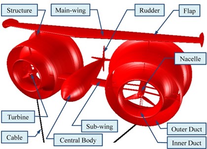
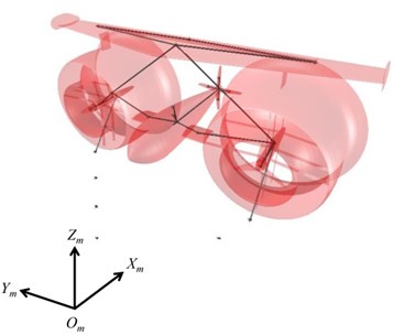
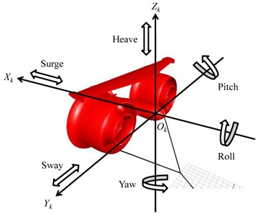
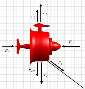
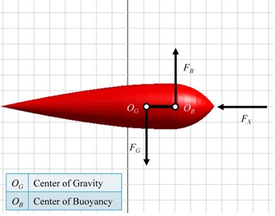
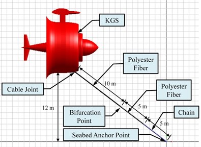
A schematic diagram of the KGS is shown in Fig. 1(a). An earth-fixed coordinate system $\left\{m\right\}$ in the KGS was indicated in MapleSim software, as shown in Fig. 1(b). The KGS comprises a cable (i.e., elastic polyester fibers and a chain), anchor, and stable floating aircraft that consists of a central body, main wing with a flap, two sub-wings, rudder, double ducts, and two direct-drive permanent magnet (PM) generators equipped with external rotors and turbines. The design concept of the double duct in the KGS involved adding inner and outer ducts to accelerate the fluid current. The KGS has several advantages such as altitude control for electric power generation or routine inspection and resistance to severe weather (e.g., typhoons, storms, and billows). If a free lift actuates on the KGS at sea, a theoretical analysis of the entire KGS must be established to maintain system stability and to change the operational altitude. In general, there are six degrees of freedom of motion in the KGS at sea with an aircraft coordinate system $\left\{k\right\}$, as shown in Fig. 2(a) (i.e., translation axes: surge, sway, and heave; and rotation axes: roll, pitch, and yaw). Several external forces, including buoyancy, gravity, hydrodynamic force (e.g., drag and lift), cable tension, and inertial force, are influential in the dynamics of the KGS, as illustrated in Fig. 2(b). The equations for force equilibrium in the surge and heave axes (i.e., translation in the $X$ and $Z$ axes) of the KGS are expressed as:

where $F_G$ is gravity, $F_B$ is buoyancy, $F_L$ is lift, $F_D$ is drag, $F_H$ is hydro-force, $F_T$ is tension ($F_{TH}$ and $F_{TS}$ are the tension in the heave and surge axes, respectively), and $F_{LD}$ is lift-induced drag.

Fig. 1a) A schematic diagram of the KGS, b) an earth-fixed coordinate system m in the KGS

a)

b)

Fig. 2a) Six degrees of freedom of the KGS at sea with an aircraft coordinate system k, b) free body diagram of the KGS

a)

b)

The force of the KGS in the sway axis (i.e., translation in the $Y$ axis) is balanced because the KGS is designed as a symmetrical structure. The impact of the aforementioned forces in six degrees of freedom at any time must be considered in the dynamic equilibrium of the KGS. In addition, the floating postures of the KGS cause changes in the magnitude of the force and moment. A suitable rudder design was assembled in back of the central body, and it could constrain the motion axes in sway, roll, and yaw. Thus, the KGS was automatically and efficiently aligned with the inflow of the Kuroshio Current. The drag analyzed and estimated in advance by using the ANSYS Fluent were generated by the current at a 0° angle of attack in front of the KGS and were approximately 177 and 62 kN in the $X$ and $Z$ axes, respectively. The force affected in the sway axis (i.e., $Y$-axis translation) and the moment rotated around the axes in roll and yaw (i.e., $X$-axis and $Z$-axis rotation) could be disregarded. The drag varied depending on the outline shape of the KGS and current speed. The total mass and buoyancy of the KGS were 1.05×10⁵ and 1.2×10⁵ kg, respectively.

3. Stability analysis and dynamic equilibrium

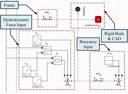
First, a rigid model architecture diagram of the central body in the KGS was created using MapleSim, as shown in Fig. 3(a). A rigid body element was adopted to represent each component of the prototype in the KGS. In other words, each component of the KGS was regarded as a different particle in three-dimensional space. The actual geometric appearance of the particle could be emerged, and the component design was imported into the software and combined with the rigid body. Moreover, the gravity and buoyancy were located at the centers of gravity and buoyancy (i.e., $O_G$ and $O_B$), respectively. If the centers of buoyancy and gravity did not match, a linkage was adopted to connect both centers. Fig. 3(b) illustrates a modeling framework of the central body in the KGS to establish the centers of gravity and buoyancy. A whole rigid model of the KGS could be built completely using a similar modeling approach.

Fig. 3a) A rigid model architecture diagram and b) a linkage connected with both centers of buoyancy and gravity of the central body in the KGS

a)

b)

The initial conditions in the KGS for simulation are at a standstill. The hydrodynamic force data simulated in the Kuroshio Current at 1.5 m/s were provided for the KGS equipped with a 4 m diameter turbine; thus, the dynamic equilibrium and stability analyses of the KGS could be performed. Weight parameters estimated using Rhino software were set on the rigid body elements in the MapleSim software according to gravity. When the KGS is fully submerged, the location of the center of gravity and buoyancy is almost overlapping. In addition, the symmetrical design configuration on both sides and the fixed rudder behind the central body could make the KGS automatically align the direction of the Kuroshio Current. Regarding buoyancy, applied world force (AWF) elements were added to input the buoyancy of all components toward the positive direction in the earth-fixed coordinate system $\left\{m\right\}$. All force element inputs were based on the earth-fixed coordinate system $\left\{m\right\}$ and did not change their directions when the rigid body elements rotated. A component weight was set as zero when an additional rigid body element that represents the center of buoyancy was established in the KGS. However, the centers of gravity and buoyancy overlapped when the rigid body element that represents the center of buoyancy was not established. As long as the buoyancy of the rigid element was input at the center of gravity, the gravity and buoyancy would be set in the simulation. According to hydrodynamic force, three-axis simulation data of the hydrodynamic force could be calculated in advance by using ANSYS Fluent. Assume that the current speed is 1.5 m/s in the simulation, inflow direction is set at a 0° angle of attack in front of the KGS, and hydrodynamic force is linear from 0 to 10 s. Drag occurs in the KGS because the flap of the main-wing redirects to lift, and the lift-induced drag increases as the angle of attack increases. Subsequently, the various AWF elements connected to the centers of gravity were adopted to input the hydrodynamic force, and the stability analysis and dynamic simulation of the KGS could be achieved. However, the KGS model in this study was divided into several rigid body elements and connected with one another. The force depending on different rigid body elements were then input in MapleSim. The postures of the KGS were changed constantly by the moment impact in the simulation. Hence, the inflow directions and KGS postures are time varying, and the continued force with a fixed magnitude and direction are not rigorous or suitable for a real case. To make the dynamic simulation in this study correspond to a real case, various forces generated by inflow impact at varied angles in the KGS were observed. The input force was changed by the inflow at a 0° angle of attack when pitch motion in the dynamic simulation appeared in the KGS.

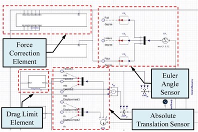
Fig. 4a) Force illustration of coordinate transformation, b) force correction of two quadratic equations, c) signal process architecture for force correction in the MapleSim software

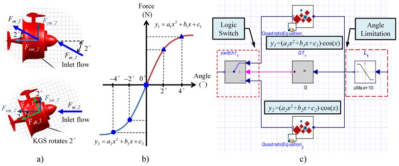
Assume that the KGS is rotated 2° counterclockwise around the pitch axis (i.e., $Y$-axis rotation), as illustrated in Fig. 4(a); the input of the inflow force in MapleSim should be a variation between –2° and 0° angles of attack and then converted into a –2° angle of attack. Moreover, accurate values for force were obtained after multiplying by $\mathrm{c}\mathrm{o}\mathrm{s}$(2°), and then the aircraft coordinate system $\left\{k\right\}$ was transformed into the earth-fixed coordinate system $\left\{m\right\}$. In this study, the current speed is assumed at 1.5 m/s. The inflow direction was respectively setup at 0°, ±2°, and ±4° angles of attack in front of the KGS, and then the hydrodynamic force of the KGS could be calculated in advance by adopting ANSYS Fluent. In order to approximate the hydrodynamic force in nonlinear regression analysis to match up real-life results, the hydrodynamic force was regressed as two quadratic equations as illustrated in Fig. 4(b). The force variation could be estimated due in different rotation angles using a direct method of interpolation, and the quadratic equations of the force variation around positive or negative pitch-axis motion in the KGS (i.e., $y_1$ and $y_2$) were obtained. Immediately after each component rotated around the pitch-axis, the force variation could be estimated using the quadratic equations by substituting the angles of the pitch-axis rotation. The force variation could be linearized due to the rotation, and two quadratic equations of the force variation around positive or negative pitch-axis motion in the KGS (i.e., $y_1$ and $y_2$) were obtained. Immediately after each component rotated around the pitch-axis, the force variation could be estimated using the quadratic equations by substituting the angles of the pitch-axis rotation. The force variation was fed back into the AWF, adding to the force at the initial value at a 0° angle of attack, and thus, the force generated by the inflow impact could be corrected with pitch-axis motion in the KGS. The signal process architecture for the force correction in MapleSim is illustrated in Fig. 4(b). The angle signal of the KGS passed through an angle limitation element, and then the force variation was modified using a logic switch. When the input signal was higher than 0, the force variation could be computed using a quadratic equation element $y_1$. By contrast, the force variation could be calculated using a quadratic equation element $y_2$. Additionally, in order to fit in with the formula of the output power in the KGS:

where ${\rho }_{sw}$ is the density of the seawater (i.e., 1025 kg/m³), $V_i$ is the angular velocity of the impeller in the KGS, $A_i$ is the disc area of the impeller, $C_P$ is the conversion power factor (i.e., the conversion efficiency). Hence, the output power of the KGS is proportional to the cube of the angular velocity of the impeller in the KGS.

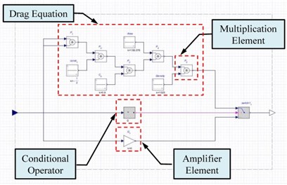
The force correction caused by the rotation in the KGS was examined, and the force variation regarding the translation in the KGS is discussed as follows: The KGS was submerged at sea, and the motion behavior in the seawater was restricted. The KGS was subjected to drag in the opposite direction when it moved to an arbitrary direction in the seawater. However, the ideal motion behavior of the rigid body in a vacuum is presented by the physical model approach in the software. Thus, drag equations must be added to the simulation framework to establish restrictions of initial conditions. The KGS was not affected by the drag in the beginning of the simulation because the KGS and seawater were both stationary in the initial state. For instance, a relative velocity was yielded between the KGS and seawater after the KGS input a fixed value of buoyancy, and thus, upward motion occurred with a uniform acceleration. This velocity value could be obtained and was substituted into the drag equations, and the drag was then added to the buoyancy. Hence, the simulated setup could precisely match realistic dynamic behavior. The KGS remained at a terminal speed to float at a constant velocity. When the gravity of the KGS was greater than the buoyancy, it could be at a terminal speed in the opposite direction to sink at a constant velocity. By revising coefficients of the drag equations, drag was obtained as the KGS moved. A signal process framework of the drag in the software is shown in Fig. 5(a). After the translation and rotation speed signals of the KGS were obtained, the logic switch could be adopted to select positive or negative speed correctly. If the speed values are positive, the KGS floats; otherwise, the KGS sinks. In addition, the speed values were substituted for the drag equations and calculated using multiplication elements. When the speed values differed from conditional operators, the signals were returned to 0 by amplifier elements. The speed signals of the KGS were passed through the drag equations for floating and sinking motion simultaneously: one signal was the drag to float or sink, and the other was 0. Thus, the net force of the gravity and buoyancy was added to the estimated drag, and then the force feedback around the heave axis was obtained. In addition, the KGS produced backward or forward drag when it moved forward or backward, but not the drag for floating and sinking motion. The hydrodynamic force data simulated in the Kuroshio Current at 1.5 m/s were provided for the KGS equipped with a 4 m diameter turbine; therefore, the dynamic simulation and stability analysis of the KGS could be achieved.

In general, the drag equation can be expressed as:

where $F_D$ is the drag (the value could be calculated in advance by using ANSYS Fluent) that was generated from the inflow impact in the KGS, $V_r$ is the speed of the KGS relative to the seawater, $C_D$ is the drag coefficient, and $A_p$ is the projection area of the KGS. Table 1 presents the parameters of the drag equations when the KGS moved upward, downward, forward, and backward.

Absolute translation sensor (ATS) and Euler angle sensor (EAS) elements were connected to the rigid elements of the gravity centers in the KGS to analyze and investigate the requirements of stability analysis and dynamic equilibrium. The modeling framework of the sensor elements are illustrated in Fig. 5(b). The displacement and velocity of the gravity centers in the KGS related to the earth-fixed coordinate system $\left\{m\right\}$ in the $X$, $Y$, and $Z$ axes could be detected from the ATS and EAS elements, respectively (i.e., the motion behavior of the six freedom degrees in the KGS: surge, sway, heave, roll, pitch, and yaw). The translation signals detected from the ATS elements passed through a drag limit element. In addition, the rotation signals detected from the EAS elements passed through a force correction element. The force and moment of the KGS could be corrected using the hydrodynamic force in the simulation.

Fig. 5a) A signal process framework of the drag, b) modeling framework of the sensor elements

a)

b)

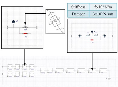
Fig. 6a) Left view and b) internal architecture diagram for modeling framework and the parameter values of the cable design

a)

b)

In addition, a rigid model architecture of a cable design connected between the KGS and seabed was constructed in the simulation. The left view of the cable design is illustrated in Fig. 6(a). The cable design was composed of elastic polyester fibers and a rigid chain to improve both characteristics of flexibility and rigidity. The KGS was setup to operate within 20 m depth of seawater, so the length of the cable design was set as 20 m. The weights per meter for the chain and polyester fiber were set as 50 kg and 20 kg in the software, respectively. The internal architecture diagram for the modeling framework and parameter values of the cable design are shown in Fig. 6(b). Moreover, three elastic polyester fibers were connected to one another by employing a $Y$-shaped configuration. Several segmented spring-damper actuating systems were adopted to design the simulation of the elastic polyester fibers. Various interval values of the spring stiffness and the damper coefficient of the polyester fibers were setup in MapleSim software. First, the smaller, middle, and lager intervals of the spring stiffness were setup as 1×10⁵ N/m, 3×10⁵ N/m, and 5×10⁵ N/m, respectively. The optimal spring stiffness could be decided on 5×10⁵ N/m through observing the responses of displacement in the KGS. Next, the damper coefficient could be adjusted in the simulation, and the optimal value was 3×10⁵ N∙s/m. The origin of the earth-fixed coordinate system $\left\{m\right\}$ (i.e., $O_m$) was set at a joint of the designed cable on the seabed. Because the chain could add the weight of an anchor system, it could not slide easily by increasing the weight and friction on the seabed. The chains would contact and park on the seabed to avoid destroying the polyester fibers if the KGS sank. Operating the KGS is easy when the elastic polyester fibers of the cable design are lighter than the floating KGS. Thus, spring stiffness, damper coefficient, and joint positions could be modified repeatedly to make the system stable in the dynamic simulation.

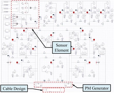
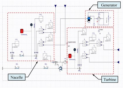
Fig. 7a) The whole system model of the KGS, b) internal modeling framework of a PM generator

a)

b)

Based on the aforementioned modeling framework creation, the whole system model of the KGS was achieved, as shown in Fig. 7(a). The origin of the earth-fixed coordinate system $\left\{m\right\}$ (i.e., $O_m$) was set to be a reference point. The initial position of the gravity center in the KGS was set at 17, 0, and 16 m. The modeling parameters were modified under different conditions for the simulation (e.g., adjustment of the spring stiffness, damper coefficients, and joint positions of the cable design). The dynamic variables of the KGS could be obtained using the ATS and EAS elements, and thus, the translation positions and rotation angles of the KGS could be determined when the dynamic equilibrium of the KGS was stable at sea. If the configuration of the KGS and cable design did not change provisionally, various spring stiffness and damper coefficients of the polyester fibers could be adjusted repeatedly to meet the requirements of the stability analysis and dynamic simulation. The polyester fibers would be elongated as soon as both the spring stiffness and damper coefficient decreased. Moreover, the KGS floating altitude and displacement variation in the heave axis were larger. Both parameters were increased, and the KGS floating altitude and displacement variation in the surge-axis become smaller. Finally, the optimal spring stiffness and damper coefficient of the polyester fibers were designated as 5×10⁵ N/m and 3×10⁵ N∙s/m in the dynamic simulation, respectively. The velocity in the surge axis (i.e., $X$ axis) of the KGS is slightly faster than that in the heave axis (i.e., $Z$ axis), and they are acceptable in the KGS.

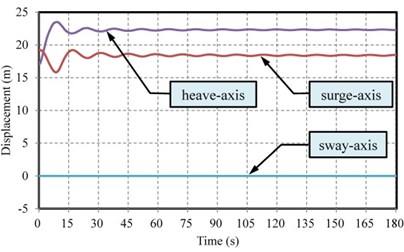
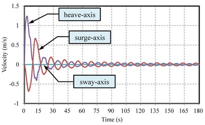
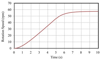
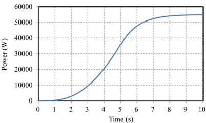
The translational motion analysis of the KGS was completed, and the posture variation in the seawater is discussed as follows: Because the top and bottom configuration design of the KGS were imbalanced, the head of the KGS constantly has a downward tendency in the flow field of the Kuroshio Current. In addition, the inflow at a 0° angle of attack was inlet in the simulation, and a negative torque around the pitch axis (i.e., $Y$ axis) was generated by an irregular distribution of up or down forces in the KGS. Thus, pitch angles were adjusted using various joint positions of the cable design when revising a system modeling process. The initial conditions of the cable joint positions were set temporarily at –1.41, ±7.5, and –4.25 m (i.e., the leading infraedge of the outer duct). However, the pitch-axis motion of the KGS was unfavorable in the dynamic simulation under the initial conditions of the cable joint positions. Different cable joint positions were simulated and verified by trial and error to obtain an optimal result. Finally, the optimal cable joint position was set at –2.2, ±7.5, and –4.25 m. In summary, the optimal spring stiffness, damper coefficients of the polyester fibers, and the cable joint positions were simulated again, using the MapleSim software. The KGS could be submerged at a stable operational altitude and horizontal posture; thus, the Kuroshio Current could flow through the turbine to generate power. This study demonstrated the internal modeling framework of a direct-drive PM generator equipped with an external rotor in the KGS that consists of a turbine rigid component, generator centrosome rigid component, and PM generator component, as shown in Fig. 7(b). Table 2 presents the specifications of the PM generator component in the KGS. In the final dynamic simulation, the time responses of displacement and velocity in the surge, sway, and heave axes (i.e., translation in the $X$, $Y$, $Z$ axes, respectively) of the KGS can be obtained by calculation and simulation, as shown in Figs. 8(a) and 8(b), respectively. The rotation speed and estimated output power of the PM generator component in the KGS can approach 57 rpm and 54.8 kW, respectively, as shown in Figs. 9(a) and 9(b).

Fig. 8Time responses of a) displacement and b) velocity in the surge, sway, and heave axes (i.e. translation in the X, Y, Z axes, respectively) of the KGS

a)

b)

Fig. 9a) Rotation speed and b) estimated output power of the PM generator component in the KGS

a)

b)

4. Conclusions

In this study, an integrated modeling framework of a novel KGS was created using MapleSim software to achieve a stability analysis and dynamic equilibrium. The approach can simplify conventional simulation processes to complete dynamic simulation quickly and efficiently and can be used to obtain the motion trajectory of the designed KGS at sea. Various parameters of spring stiffness, damper coefficients, and joint positions of cable design that affect the motion were simulated, and different modeling frameworks were modified to meet the requirements of dynamic equilibrium and stability analysis. The optimal spring stiffness and damper coefficient of the polyester fiber in cable design were designated as 5×10⁵ N/m and 3×10⁵ N∙s/m in the simulation, respectively. In addition, the optimal joint position, which is relative to the leading infraedge of the outer duct, was set at 2.2 m along the negative surge axis. Both translation ranges in the surge and heave axes could be approximated to 0.5 m, and the estimated output power of the designed permanent magnet generator in the KGS exceeded 54.8 kW. Furthermore, the simulation method of stability analysis and dynamic equilibrium can be applied in all types of generator system.