A finite element model in a form of structural dynamic equation for the transient analysis of pressure in pipelines

Barauskas, Rimantas; Kriščiūnas, Andrius; Blažauskas, Tomas

doi:10.21595/jve.2016.16609

Journal of Vibroengineering

Browse Journal

Submit article

Published: 31 March 2016

Check for updates

A finite element model in a form of structural dynamic equation for the transient analysis of pressure in pipelines

Rimantas Barauskas¹

Andrius Kriščiūnas²

Tomas Blažauskas³

^{1, 2, 3}Kaunas University of Technology, Kaunas, Lithuania

Corresponding Author:

Rimantas Barauskas

Cite the article Download PDF

Downloads 1201

Abstract

The finite element model of transient pressure pulse propagation in a pipeline is presented in the form of the standard structural dynamic equation, which combines steady flow analysis for obtaining the initial conditions of the flow in the form of pressures and flow rates and non-linear dynamic analysis by using explicit numerical integration techniques. Three options of simplification of governing equation set have been analyzed. At low values of steady flow speed many non-linear and convection terms could be omitted, while at the flow speeds comparable with the wave propagation speed the full equation system has been analyzed. The full equation system analysis involves the techniques ensuring corrections of the initial conditions and of the nodal flow rate balance. The investigated pipelines may contain large number of branches and loops. Parts of large pipelines are analyzed as separate sub-models by employing non-reflecting boundary conditions at the cut boundaries. Properties of pressure pulse front degradation as it propagates through branching points of the pipeline can be examined.

1. Introduction

The basic mathematical models of fluid transients have been formulated long since. They were used generally to research the water-hammer problems that occur in a pipeline (either upstream or downstream from a valve) when sudden closure of a valve happens [1]. The solutions for pipelines of uncomplicated geometric configuration could be obtained analytically. In more complicated situations the method of characteristics (MOC) has to be applied that was originally developed for quick transients in liquid pipelines. The development of efficient numerical algorithms for wave, vibration and pulse propagation analysis in pipelines steadily engages numerous researchers and remains among significant problems of computational fluid dynamics. Though MOC is still used up-to-now to solving fluid transients problems, it has certain underlying shortcomings, such as the strict adherence to the relationship of the time steps against the model discretization steps along the lengths of the pipes. Many different sonic velocity values over a pipe network are inherent for the fluid flow networks constituted of pipes of many different diameters, and the elastic properties of the pipe make influence on the equivalent bulk modulus of the fluid. For example, in a heating network of a city sonic velocities in different pipeline segments may vary ~10-40 %. This means that for fixed length increments the required time step is different as the flow along different pipes of the network is investigated.

As alternatives, the numerical schemes based on the finite difference method, the finite volume method and the method of lines have been traditionally employed. In [2] Eulerian-based and Lagrangian-based methods for modeling pressure transients have been compared. In [3] finite difference-based efficient second order Godunov-type numerical method has been developed for simulation of the water-hammer problem in piping, in which fast Riemann solver has been constructed. In [4] performances of method of lines and finite difference method were tested from the viewpoints of solution accuracy and solution time. An implicit finite difference method has been described in [5], which is valid for both quick and slow transients, as well as, for steady flows.

Application of the finite element method (FEM) to pipeline fluid flow transient analysis was always attractive because of the analogy of the structure of the computational model to the real system. Moreover, it allows to use regular structural dynamics analysis tools for solving pipeline transients and vibration problems, as well as, to develop the coupled models based on fluid-structure interaction for pipeline pressure and structural vibration analysis. Many engineers should regard the finite element model as the most expedient one to presentation the heterogeneous structures of large pipe networks. However, the FEM scheme for pipeline flow cannot be directly gained by applying the Galerkin procedure to uni-dimensional compressible flow equations and using both pressure and flow velocity as nodal variables. The difficulty to be confronted here is that the flow velocities have to satisfy the condition of the flow rate balance at the pipe intersection nodes rather than the nodal value compatibility condition. Numerous constraint equations should be taken into account. Several finite element schemes suited for fluid and gas flow transients have been reported [6-9]. In early work [6] a general computational technique has been developed for the study of uniaxial linear vibration of compressible fluids in piping systems. The approach (based of finite element mobility method) was similar to the stiffness method in structural mechanics finite element models. The elements included in the model comprised finite and semi-infinite fluid columns, intermediate and boundary mass-spring-damper systems, cavity springs and modal bodies. A finite element model of the flow in the pipe with laminar frequency-dependent friction developed in [7] retained the accuracy of the MOC. Based on the finite element model, an electronic analogue methodology has been utilized to solving the problem of fluid transients. Pressures, velocities and frequency-dependent friction were used as the nodal variables. The formulation of the fluid-structure interaction presented in [8] included axial vibration model of the pipe aiming at better estimating the relative velocity of the fluid against the pipe wall. The model was based on the assumptions of linear elasticity, no buckling, negligible radial inertia, and low Mach number. Most reported finite element models of transient pipe flow were based on simplified systems of governing equations, in which convection and (or) non-linear terms can be neglected. An extensive/general characterization of different options of existing transient models and approaches to their solution has been provided in [9].

The mathematical form of obtained finite element model heavily depends of the selected type of transformation of the set of basic equations. Subject to the degree of simplification with respect to the set of basic equations, the equations of the fluid-structure interaction will be linear or, quite generally, non-linear. Possible transformations of the basic equation set could come out in the differential equations of first or second order.

The approach developed in this work presents the finite element model as a standard structural dynamic equation in terms of pressure variables and their first and second-order time derivatives. If convection terms could be omitted, the flow rate variables will appear only in non-linear damping terms of the equation. The finite element model is generated by using both first order form functions for pressure field approximation within the finite element, and the zero-order flow rate field approximation. Though originated from a rather simple idea to transform the pipeline pressure vibration problem to the form most relevant to the structural dynamic equation, the study considers also models, in which the complete model equation set is handled, without no simplifications of the governing equations. The latter is important in the case of highly elastic pipes with low effective values of the combined bulk modulus, which takes into account both pipe wall elasticity and fluid compressibility. In such situations the velocity of the pressure wave propagation is much lower than within rigid pipes, and can be comparable with the fluid flow velocity. The problems of this kind may be encountered, particularly, in biomedical simulations such as blood flow in blood vessels with highly elastic walls.

Also other advantages of the presented form of equations may be anticipated. An inherent hindrance encountered in the explicit analysis of fast transients by using finite element models is associated with the distortion of the short wavelength pulse simulated in a discrete mesh. The extent of distortion grows rapidly with time as the distance travelled by the pulse comprises a considerable number of lengths of the pulse. A substantial source of distortions of the pulse shape seems to be the phase error produced by the model. A regular approach to minimization of the phase errors has been developed earlier, in [10-11], where the mass and stiffness matrices of elastic component domains have been synthesized in such a way that after assembling the component domain matrices to a larger model the convergence of modal frequencies should be as high as possible. The approach seems to be relevant and directly applicable to the models developed in this work.

2. Basic equations

Let us consider differential element $d x$ of the fluid in the pipe of uniform cross-section. The basic set of uni-dimensional flow equations, which contains the continuity equation and the linear momentum conservation equation reads as:

1

\{\begin{array}{l} \frac{\partial m}{\partial t} + \frac{\partial (m v)}{\partial x} = 0, \\ \frac{\partial (m v)}{\partial t} + \frac{\partial (m v^{2})}{\partial x} + A \frac{\partial p}{\partial x} + \frac{f}{D} \frac{m v |v|}{2} + m g \sin a = 0, \end{array}

where $p$ is the fluid pressure, $m = ρ A$ is the mass of the fluid of mass density $ρ$ per unit length of the pipe of cross-sectional area $A$ , $v$ are the velocity of the fluid flow, $a$ is the angle of the pipe to against the horizontal, $g$ is the free-fall acceleration, $f = 0.3614 / \sqrt[4]{R e}$ is the friction coefficient for turbulent flow, where $R e$ is the Reynolds number.

Having the differentiation in Eq. (1) is carried out, the obtained partial derivatives are combined to material derivatives and provide the following relation:

2

\{\begin{array}{l} \frac{1}{m} \frac{d m}{d t} + \frac{\partial v}{\partial x} = 0, \\ \frac{\partial v}{\partial t} + v \frac{\partial v}{\partial x} + \frac{1}{ρ} \frac{\partial p}{\partial x} + \frac{f}{D} \frac{v |v|}{2} + g \sin a = 0, \end{array}

where $d / d t$ denotes the material derivative expressed as $d m / d t = \partial m / \partial t + v \partial m / \partial x$ .

The compressibility of the flow is taken into account by means of the relation:

3

\frac{d p}{\tilde{K}} = \frac{d m}{m},

where $\tilde{K} = K {(1 + K D / h E)}^{- 1}$ is the equivalent bulk modulus of the pipe, which combines the bulk stiffness of the fluid and the radial expansion stiffness of the pipe, $K$ is the bulk modulus of the fluid, $E$ is the stiffness modulus of the pipe material, $D$ , $h$ are the diameter and wall thickness of the pipe [1].

Now Eq. (3) is substituted into Eq. (2), and material derivative is replaced by partial derivatives as:

4

\{\begin{array}{l} \frac{\partial p}{\partial t} + v \frac{\partial p}{\partial x} + \tilde{K} \frac{\partial v}{\partial x} = 0, \\ \frac{\partial v}{\partial t} + v \frac{\partial v}{\partial x} + \frac{1}{ρ} \frac{\partial p}{\partial x} + \frac{f}{D} \frac{v |v|}{2} + g \sin a = 0 . \end{array}

Notice that $1 / ρ = A / m$ , therefore the Eq. (4) does not contain the cross-sectional area term any more. In the following derivations it is reasonable to assume the value of cross-sectional area $A$ as constant and to calculate the density of the fluid at each moment of time as:

5

ρ = ρ_{0} (1 + \frac{p - p_{0}}{\tilde{K}}),

by taking into account the combined elasticity of the fluid and of the pipe wall, where $p_{0}$ is the reference pressure at which the density of the fluid is $ρ_{0}$ .

Transformation of the Eq. (4) to the structural dynamic equation form is carried out as follows. The derivative $\partial v / \partial x$ is calculated from Eq. (4) as:

6

\frac{\partial v}{\partial x} = - \frac{1}{\tilde{K}} (\frac{\partial p}{\partial t} + v \frac{\partial p}{\partial x}),

and substituted into Eq. (4). Further, Eq. (4.1) is differentiated with respect to time, Eq. (4.2) and Eq. (5) are differentiated with respect to $x$ and combined together in order to eliminate $\partial^{2} v / \partial x \partial t$ and $\partial ρ / \partial x$ . The resulting equation system reads as:

7

\{\begin{array}{l} [\begin{array}{l} \frac{\partial^{2} p}{\partial t^{2}} - (\frac{\tilde{K}}{ρ} - v^{2}) \frac{\partial^{2} p}{\partial x^{2}} + (\frac{f |v|}{D} - \frac{2 v}{\tilde{K}} \frac{\partial p}{\partial x} - \frac{1}{\tilde{K}} \frac{\partial p}{\partial t}) \frac{\partial p}{\partial t} \\ + (\frac{f v |v|}{2 D} - g \sin a + (\frac{ρ_{0}}{ρ^{2}} - \frac{1}{ρ} - \frac{v^{2}}{\tilde{K}}) \frac{\partial p}{\partial x}) \frac{\partial p}{\partial x} + 2 v \frac{\partial^{2} p}{\partial x \partial t} = 0 \end{array}], \\ \frac{\partial v}{\partial t} = \frac{v}{\tilde{K}} \frac{\partial p}{\partial t} - (\frac{1}{ρ} - \frac{v^{2}}{\tilde{K}}) \frac{\partial p}{\partial x} - \frac{f}{D} \frac{v |v|}{2} - g \sin a . \end{array}

Equation system Eq. (7) preserves all the features of the model given by the original equation system Eq. (1). Later in the text we will refer to Eq. (7) as the full equation system, or equation Type 3.

At low values of flow velocity compared to wave propagation speed $\sqrt{\tilde{K} / ρ}$ and nearly incompressible fluid, the simplified version of Eq. (7) is obtained by omitting non-linear and convection terms as:

8

\{\begin{array}{l} \frac{\partial^{2} p}{\partial t^{2}} + \frac{f |v|}{D} \frac{\partial p}{\partial t} - \frac{\tilde{K}}{ρ_{0}} \frac{\partial^{2} p}{\partial x^{2}} = 0, \\ \frac{\partial v}{\partial t} = - \frac{1}{ρ_{0}} \frac{\partial p}{\partial x} - \frac{f}{D} \frac{v |v|}{2} - g \sin a . \end{array}

Eq. (8) contains all the terms traditionally used for water-hammer calculations, where the pressure wave propagation speed exceeds the flow velocity many times. However, Eq. (8.1) enables to obtain the finite element formulation in the standard form of structural dynamic equation, provided that appropriate approximation orders for pressure and velocity variables is selected. The coupling of Eq. (8.1) to Eq. (8.2) can be observed within the damping term only, which is linearly proportional to the absolute value of the flow velocity. At low values of flow velocities, the damping does not essentially influence the basic dynamic properties of the system. Later in the text we refer to Eq. (8) as equation Type 1.

Another option of the simplified equation, which includes the convection and fluid compressibility terms, reads as:

9

\{\begin{array}{l} \frac{\partial^{2} p}{\partial t^{2}} + \frac{f |v|}{D} \frac{\partial p}{\partial t} - (\frac{\tilde{K}}{ρ} - v^{2}) \frac{\partial^{2} p}{\partial x^{2}} + (\frac{f v |v|}{2 D} - g \sin a) \frac{\partial p}{\partial x} + 2 v \frac{\partial^{2} p}{\partial x \partial t} = 0, \\ \frac{\partial v}{\partial t} = \frac{v}{\tilde{K}} \frac{\partial p}{\partial t} - (\frac{1}{ρ} - \frac{v^{2}}{\tilde{K}}) \frac{\partial p}{\partial x} - \frac{f}{D} \frac{v |v|}{2} - g \sin a . \end{array}

Eq. (9) have been obtained from Eq. (7) by omitting the non-linear pressure terms. As demonstrated by numerical examples, in many practical situations the differences between solutions of Eq. (7) and Eq. (9) are rather negligible, whereas Eq. (8) tends to produce significant inadequacies at higher flow velocities, as well as, at lower values of equivalent bulk modulus $\tilde{K}$ . Later in the text we refer to Eq. (9) as equation Type 2.

3. Finite element model

We develop the finite element formulation on the base of equation system Eq. (7). The formulations for Eq. (8) and Eq. (9) can be easily obtained by omitting the corresponding terms in the finite element expressions.

3.1. Steady flow

Transient analysis of pressure vibrations in the pipeline is started by assuming the steady flow solution as an initial condition. In the case of pipeline flow the compatibility condition of nodal values of the finite elements is valid for pressure terms only. The flow mass rates at each node satisfy the balance condition. We transform the equation to the form where flow rates are the right-hand side terms of the equations and are added-up to zeros or to external flow rate sources as the structural equations are assembled. Constant values of flow rates and linear distributions of pressure values over finite elements are assumed. At the first stage the steady flow solution is obtained by using Eq. (7.2), in which time-dependent terms are omitted as:

10

(\frac{1}{ρ} - \frac{v^{2}}{\tilde{K}}) \frac{\partial p}{\partial x} + \frac{f}{D} \frac{v |v|}{2} + g \sin a = 0 .

Two equations necessary to describing the flow rate balance over the finite element are obtained by integrating Eq. (10) from 0 to $L$ and from $L$ to 0 as:

11

\{\begin{matrix} \int_{0}^{L} ((\frac{1}{ρ} - \frac{v_{e}^{2}}{\tilde{K}}) \frac{\partial p}{\partial x} + \frac{f}{D} \frac{v |v|}{2} + g \sin a) d x = 0, \\ \int_{L}^{0} ((\frac{1}{ρ} - \frac{v_{e}^{2}}{\tilde{K}}) \frac{\partial p}{\partial x} + \frac{f}{D} \frac{v |v|}{2} + g \sin a) d x = 0 . \end{matrix}

The following finite element equations are obtained:

12

\{\begin{matrix} \frac{2 D}{f L} (A^{2} ρ - \frac{w_{e}^{2}}{\tilde{K}}) (p_{i} - p_{j}) + \frac{2 D A^{2} ρ}{f L} p^{*} - \frac{2 D A^{2} ρ^{2} g}{f L} ∆ z = w_{i} |w_{i}|, \\ \frac{2 D}{f L} (A^{2} ρ - \frac{w_{e}^{2}}{\tilde{K}}) (p_{j} - p_{i}) - \frac{2 D A^{2} ρ}{f L} p^{*} + \frac{2 D A^{2} ρ^{2} g}{f L} ∆ z = w_{j} |w_{j}|, \end{matrix}

where $p^{*}$ is the pressure created by the pump in case the pump is present within the finite element, $∆ z = z_{j} - z_{i}$ is the increment of height along the finite element, $w = A ρ v$ is the mass rate of the flow within the finite element and $w_{i}$ , $w_{j}$ are the nodal values of the flow rate. Obviously, over a single finite element $w = w_{i} = - w_{j}$ .

The non-linear finite element equation is obtained from Eq. (12) as:

13

\{\begin{array}{l} s g n (C) \sqrt{|C|} \sqrt{\frac{2 D}{f L} (A^{2} ρ - \frac{w_{e}^{2}}{\tilde{K}})} = w_{i}, \\ - s g n (C) \sqrt{|C|} \sqrt{\frac{2 D}{f L} (A^{2} ρ - \frac{w_{e}^{2}}{\tilde{K}})} = w_{j}, \end{array}

where $C = p_{i} - p_{j} + p^{*} - ρ g ∆ z$ .

The tangential matrix of the finite element reads as:

14

[K_{T}^{e}] = \sqrt{\frac{D}{2 f L |C|} (A^{2} ρ - \frac{w_{e}^{2}}{\tilde{K}})} [\begin{matrix} 1 & - 1 \\ - 1 & 1 \end{matrix}] .

Appropriate structural vectors and matrices are assembled by using element Eq. (13) and tangential matrices Eq. (14), and standard Newton-Raphson solution procedure is carried out for obtaining the steady flow solution. Unknown values of element flow rates, which are present in Eqs. (13), (14), are updated at every Newton-Raphson iteration as $w_{e}^{(n)} = w_{e}^{(n - 1)}$ , where $n$ is iteration number. One should notice that the steady flow solution procedure cannot be started at zero initial approximation. For a horizontal pipe elements value $C$ at the first iteration is zero, therefore relation Eq. (14) is undefined. A reasonable non-zero initial approximation could be obtained by using the linear version of Eq. (13). At zero iteration the linear problem is solved, in which the right-hand side terms $w_{i} |w_{i}|$ , $w_{j} |w_{j}|$ of Eq. (13) are replaced by $w_{i}$ , $w_{j}$ , and $w_{e} = 0$ is assumed.

3.2. Dynamic equations of the finite element

Equations of uni-dimensional finite element of length $L$ are obtained by applying the Galerkin weighted residual formulation to the Eq. (7.1) as:

15

A \int_{0}^{L} {[N]}^{T} (\frac{\partial^{2} p}{\partial t^{2}} - (\frac{\tilde{K}}{ρ} - v_{e}^{2}) \frac{\partial^{2} p}{\partial x^{2}} + (\frac{f |v_{e}|}{D} - \frac{2 v_{e}}{\tilde{K}} \frac{\partial p}{\partial x} - \frac{1}{\tilde{K}} \frac{\partial p}{\partial t}) \frac{\partial p}{\partial t}

+ (\frac{f v_{e} |v_{e}|}{2 D} - g \sin a + (\frac{ρ_{0}}{ρ^{2}} - \frac{1}{ρ} - \frac{v_{e}^{2}}{\tilde{K}}) \frac{\partial p}{\partial x}) \frac{\partial p}{\partial x} + 2 v_{e} \frac{\partial^{2} p}{\partial x \partial t}) d x = 0,

where ${[N]}^{T} = [1 - x / L, x / L]$ the form function matrix of the element, which is used for interpolation of pressure in terms of nodal variables as $p (x) = [N] \{P^{e}\}$ .

The zero-order approximation for the fluid velocity, $v_{e}$ , and mass density, $ρ$ , means that the average values within a single finite element are used. In Eq. (15) the term containing $\partial^{2} p / \partial x^{2}$ is integrated by parts as follows:

- A \int_{0}^{L} {[N]}^{T} (\frac{\tilde{K}}{ρ} - v_{e}^{2}) \frac{\partial^{2} p}{\partial x^{2}} d x = {- A (\frac{\tilde{K}}{ρ} - v_{e}^{2}) {[N]}^{T} \frac{δ p}{δ x}|}_{0}^{L} - A (\frac{\tilde{K}}{ρ} - v_{e}^{2}) \int_{0}^{L} \frac{\partial {[N]}^{T}}{\partial x} \frac{\partial p}{\partial x} d x

= {- A (\frac{\tilde{K}}{ρ} - v_{e}^{2}) {(\frac{1}{ρ} - \frac{{v_{e}}^{2}}{\tilde{K}})}^{- 1} (- \frac{f}{D} \frac{v_{e} |v_{e}|}{2} - g \sin a) {[N]}^{T}|}_{0}^{L}

- A (\frac{\tilde{K}}{ρ} - v_{e}^{2}) \int_{0}^{L} \frac{\partial {[N]}^{T}}{\partial x} \frac{\partial [N]}{\partial x} d x \{P^{e}\},

where value $δ p / δ x = {(1 / ρ - v_{e}^{2} / \tilde{K})}^{- 1} (- ρ_{0} f v |v| / D 2 - ρ_{0} g \sin a)$ is substituted form Eq. (10) by assuming $\partial v / \partial t = 0$ . It ensures that the investigated transient process starts at the initial conditions described by steady flow pressures and velocities.

Finally, the finite element equations read as:

16

\{\begin{array}{l} [M^{e}] \{{\ddot{P}}^{e}\} + [C^{e} ({\dot{P}}^{e}, P^{e})] \{{\dot{P}}^{e}\} + [K^{e} (P^{e})] \{P^{e}\} + \{Q^{e}\} = 0, \\ {\dot{v}}_{e} = G, \end{array}

where:

[M_{(3)}^{e}] = A \int_{0}^{L} {[N]}^{T} [N] d x = \frac{A L}{3} [\begin{matrix} 1 & \frac{1}{2} \\ \frac{1}{2} & 1 \end{matrix}] \approx \frac{A L}{2} [\begin{matrix} 1 & 0 \\ 0 & 1 \end{matrix}],

[C_{(3)}^{e}] = (A L (\frac{f |v_{e}|}{D} - \frac{2 v}{\tilde{K}} \frac{p_{e 2} - p_{e 1}}{L} - \frac{1}{\tilde{K}} \frac{{\dot{p}}_{e 1} + {\dot{p}}_{e 2}}{2}) [\begin{matrix} \frac{1}{2} & 0 \\ 0 & \frac{1}{2} \end{matrix}] + A v_{e} [\begin{matrix} - 1 & 1 \\ - 1 & 1 \end{matrix}]),

[K_{(3)}^{e}] = \frac{A}{L} (\frac{\tilde{K}}{ρ} - v_{e}^{2}) [\begin{matrix} 1 & - 1 \\ - 1 & 1 \end{matrix}]

+ \frac{A}{2} (\frac{f v_{e} |v_{e}|}{2 D} - g \sin a + (\frac{ρ_{0}}{ρ^{2}} - \frac{1}{ρ} - \frac{v_{e}^{2}}{\tilde{K}}) \frac{p_{e 2} - p_{e 1}}{L}) [\begin{matrix} - 1 & 1 \\ - 1 & 1 \end{matrix}],

\{Q_{(3)}^{e}\} = A \tilde{K} (\frac{p^{*}}{L} - \frac{f v_{e} |v_{e}|}{2 D} - g \sin a) \{\begin{matrix} 1 \\ - 1 \end{matrix}\},

G_{(3)}^{e} = \frac{v_{e}}{\tilde{K}} \frac{{\dot{p}}_{1} + {\dot{p}}_{2}}{2} - (\frac{1}{ρ} - \frac{v_{e}^{2}}{\tilde{K}}) \frac{p_{2} - p_{1}}{L} - \frac{f}{D} \frac{v_{e} |v_{e}|}{2} - g \sin a^{e},

where $p^{*}$ is the pressure created by a pump, if the pump works within the finite element. Bottom index „(3)“ indicates that the matrices have been obtained by using full equation set of Type 3 (Eq. (7)).

In the case of the simplified set of governing equations Type 1, the relations Eq. (16) become much simpler and read as:

17

[M_{(1)}^{e}] \approx \frac{A L}{2} [\begin{matrix} 1 & 0 \\ 0 & 1 \end{matrix}], [C_{(1)}^{e}] = \frac{A L f |v_{e}|}{2 D} [\begin{matrix} 1 & 0 \\ 0 & 1 \end{matrix}], [K_{(1)}^{e}] = \frac{A}{L} [\begin{matrix} 1 & - 1 \\ - 1 & 1 \end{matrix}],

\{Q_{(1)}^{e}\} = A \tilde{K} (\frac{p^{*}}{L} - \frac{f v_{e} |v_{e}|}{2 D} - g \sin a) \{\begin{matrix} 1 \\ - 1 \end{matrix}\},

G_{(1)}^{e} = \frac{v_{e}}{\tilde{K}} \frac{{\dot{p}}_{1} + {\dot{p}}_{2}}{2} - \frac{p_{2} - p_{1}}{ρ_{0} L} - \frac{f}{D} \frac{v_{e} |v_{e}|}{2} - g \sin a^{e} .

Element Eq. (16.1) are assembled to structural equations, and Eq. (16.2) are solved for each element separately. Here, we should notice that there are no algebraic relations employed in Eq. (17), which ensure the flow mass rate balance condition at the nodes of adjacent elements. In some cases, during the time integration process the element mass rates summed together at each node may give the values, which „drift away” from correct zero values. The ways to preventing such inaccuracies will be discussed in the next subsection.

The well-known non-reflecting boundary condition [12] may be applied at cut-off boundaries of the analyzed part of the pipeline as:

18

\sqrt{\frac{\tilde{K}}{ρ}} \frac{\partial p}{\partial x} + \frac{\partial p}{\partial t} = 0 .

As model equations contain convection terms, the higher order numerical integration schemes should be applied. In his work all examples were calculated by using MATLAB function ode23tb suited to solving stiff differential equations.

3.3. Correction terms

Two noteworthy situations may occur while applying the proposed finite element scheme.

The first situation is related to the evaluation of the steady flow initial condition. As mentioned before, the steady flow was calculated by using model Eqs. (13), (14), which was based on the second equation of Eq. (2) only. Another form of the same Eq. (16.2), in which time-dependent terms are assumed to be zeros. The dynamic response is calculated by using both Eq. (16). The steady flow initial conditions, which were calculated to answer Eq. (16.2) only, have to meet also Eq. (16.1). This is really so for simplified equation set Type 1, however, the first equation is not satisfied exactly if equation Types 2 and 3 are used. This may induce an artificial initial disturbance, which results in undesirable numerical noise in the solution of the pressure vibration. The easiest way to avoid this could be the integration of finite element model equations in time without any external excitation terms. After certain time of integration, the corrected equilibrium situation is achieved as the result of the damped transient vibration process. Artificial damping could be applied in order to force quicker establishment of equilibrium. The new steady equilibrium state is assumed to be an initial condition for subsequent transient calculations.

Another way to achieve the same result is purely algebraic. By neglecting all time-dependent terms in Eq. (16) and assuming initial disturbances as zero, let us express nodal pressure $p_{e 2}$ from Eq. (16.2) and substitute into Eq. (16.1). The residual will be the equilibrium correction term, which has to be subtracted from Eq. (16.1) during each subsequent integration step. Expressions are obtained rather cumbersome and we do not present them here. A proper way used in this work was to perform all the derivation by using symbolic mathematics software and to obtain the necessary terms of the formulae as fragments of the program source code.

The second problematic situation is related with the “drifting away” situation from the nodal mass rate balance condition, while performing the subsequent time integration steps. As demonstrated by numerical examples, the drift is very small in the case of nearly incompressible flows; however, it may become considerable where the flow compressibility is significant. The remedy applied by us was based on calculation of minimum corrections of flow rates within elements. The applied corrections should ensure the nodal flow mass rate balance condition at each time step. This is performed by transforming Eq. (16.2) into finite element equation form of first approximation order as:

19

- [\begin{matrix} \frac{2 D}{f_{e} |v_{e}|} & 0 \\ 0 & \frac{2 D}{f_{e} |v_{e}|} \end{matrix}] \{\begin{matrix} {\dot{w}}_{e} + {\dot{w}}_{e}^{*} \\ {\dot{w}}_{e} + {\dot{w}}_{e}^{*} \end{matrix}\}

\approx - \{\begin{matrix} \frac{v L}{\tilde{K}} \frac{\partial p_{1}}{\partial t} + \frac{2 D A ρ_{e}}{L f_{e} |v_{e}|} (\frac{1}{ρ} - \frac{v^{2}}{\tilde{K}}) (p_{i} - p_{j}) - \frac{2 D A ρ}{L f_{e} |v_{e}|} g ∆ z \\ \frac{v L}{\tilde{K}} \frac{\partial p_{2}}{\partial t} + \frac{2 D A ρ_{e}}{L f_{e} |v_{e}|} (\frac{1}{ρ} - \frac{v^{2}}{\tilde{K}}) (p_{j} - p_{i}) + \frac{2 D A ρ}{L f_{e} |v_{e}|} g ∆ z \end{matrix}\} + \{\begin{matrix} w_{i} \\ w_{j} \end{matrix}\},

where $v_{e}$ , $w_{e}$ are averaged flow velocity and mass rate within the element, ${\dot{w}}_{e}^{*}$ is the sought correction of element flow mass rate, and $w_{i}$ , $w_{j}$ are nodal flow mass rates, which have to answer the nodal flow mass rate balance condition. As element Eq. (19) are assembled to the structural equation, the nodal values of flow mass rates (the rightmost term in Eq. (19)) add up to zeros or to prescribed external nodal flow rate values. We have to ensure the satisfaction of the assembled equation by applying minimum corrections ${\dot{w}}_{e}^{*}$ . The conditional optimization problem is formulated as:

20

\{\begin{array}{l} m i n \frac{1}{2} {\{{\dot{w}}_{e l}^{*}\}}^{T} \{{\dot{w}}_{e l}^{*}\}, \\ [R] (\{{\dot{w}}_{e l}\} + \{{\dot{w}}_{e l}^{*}\}) = \{{\dot{w}}_{n}\}, \end{array}

where $\{{\dot{w}}_{n}\}$ – assembled right-hand sides of element Eq. (19), $\{{\dot{w}}_{e}\}$ – vector containing flow mass rates time derivatives of all elements, $\{{\dot{w}}_{e}^{*}\}$ – vector containing corrections of flow mass rates time derivatives of all elements, $[R]$ – matrix assembled from left-hand sides of Eq. (19).

The solution of Eq. (20) reads as:

21

\{{\dot{w}}_{e l}^{*}\} = {[P]}^{T} {([P] {[P]}^{T})}^{- 1} ([P] \{{\dot{w}}_{e l}\} - \{{\dot{w}}_{n}\}) .

Implementation of Eq. (21) during each time step of the integration scheme is resource consuming, if the pipeline is large. Fortunately, it is not necessary in the case of nearly incompressible flows, such as water supply or heating pipelines. It may appear as enough to apply the correction procedure each tenth or even several more steps.

The correction may work poorly in the case of pipelines containing segments, where nearly zero flow rates may occur. In such situations the left-hand side matrix of Eq. (20) may become indefinite.

4. Numerical results

Verification of the model is carried out by analyzing its behavior in simple situations, the properties of solutions of which are basically known ahead. The results of numerical experiments provided in this section illustrate the behavior of the proposed finite element scheme when applied to the pulse propagation along a uniform pipe at different flow rates and different sonic velocities. As a test example a sample pipe of 600 mm diameter, wall thickness 8 mm and 720 m length was selected. At each numerical experiment the calculations start from the steady flow situation, which is obtained by solving numerically the steady flow problem Eq. (13) at prescribed input flow rates.

Let us consider the water flow in the pipe. The parameters used are Young’s modulus $E =$ 2.1×10¹¹ Pa of the pipe material, water bulk modulus $K =$ 2.2×10⁹ Pa, mass density $ρ =$ 995 kg/m³, dynamic viscosity $μ =$ 0.547×10^-3 (N×s)/m². The speed of the pressure wave in such a pipe is 1112.7 m/s. Two situations were analyzed where input volumetric rates were 400 m³/h and 40000 m³/h, the corresponding pressure drops along the pipe at the steady flow situation were 0.01146 MPa and 3.62 MPa, corresponding flow mass rates were $w =$ 110.56 kg/s and w=110.56 kg/s, flow velocities $v =$ 0.3928 m/s and. $v =$ 39.28 m/s The obtained almost commensurate ratios of values obtained in both situations indicate that the fluid is nearly incompressible, and the flow velocity along the pipe is practically constant. The excitation pressure pulse is generated at the left hand end of the pipe as the pressure overshoot 10⁵ Pa of half-cosine pulse front of duration 0.15 s is applied.

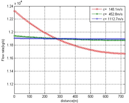
Fig. 1(a) presents the distribution of dynamic pressure values (i.e. the difference of pressures obtained during pressure pulse propagation from the values of obtained at the steady flow situation) along the pipe at time moment $t =$ 2 s at two different steady flow velocity values 0.39 m/s and 39 m/s. The pressure at the right-hand end of the pipe is assumed to be fixed and equal to the pressure at the steady flow situation. The curves illustrate that the equations of all considered equation Types 1, 2 and 3 provide practically identical results at low velocities of the steady flow. However, at higher steady flow velocities the advection terms in equations Types 2 and 3 condition necessary corrections to the resulting velocity of the pulse propagation. This velocity becomes higher than calculated by using the equation Type 1 as the pulse is propagating downstream, and lower – in the upstream direction. This can be observed in Fig. 1(b), where screenshots of the shape of the pressure pulse travelling downstream from the left-hand end, and then reflected from the right hand end and travelling upstream along the pipe are superimposed in the same picture. It is obvious that the advection terms shouldn’t be neglected if the duration of the integration process is much larger than the pulse duration. The disparities among solutions obtained by using equations Types 2 and 3 are rather negligible at all considered steady flow velocities. The slight waviness of the pressure curve that follows the pulse front is caused by the numerical noise, which is underlying for wave equation solutions obtained in discrete meshes. Such errors can be reduced by using shorter element or by applying the generalized mass matrices instead of the lumped ones [10].

Fig. 1Distribution of dynamic pressure values along the pipe at moments of time t= 2 s at two different steady flow velocity values 0.39 m/s and 39 m/s

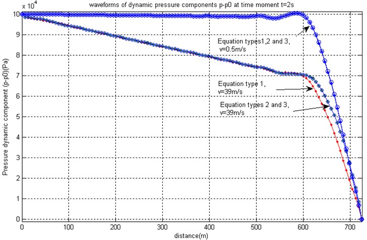
a) Pressure pulses at steady flow velocities 0.39 m/s and 39 m/s obtained by using equation Types 1, 2, and 3

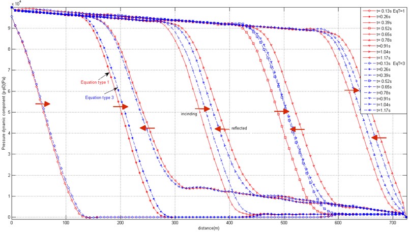
b) Superimposed screenshots of propagating and reflected pressure pulse obtained by using equation

If the speed of the wave propagation exceeds many times the speed of the steady flow, all equation types provide very close results. In such cases equation Type 1 may be used as a base for pressure pulse propagation finite element models and flow rate balance correction terms can be neglected. The model also requires no static correction terms, therefore the finite element model is simple and close to linear. The only non-linear term is the damping term, which includes the product of pressure and flow velocity. However, at low values of dynamic viscosity the basic dynamic properties of the pulse propagation are governed by stiffness and inertia terms of the model. The approach for the treatment of the model is close to that applied to structural dynamic equations.

The picture becomes different as the speed of the pressure wave propagation becomes comparable with the flow velocity one. Consider the situation where the speed of the pressure wave propagation along the pipe is 148.1 m/s, and dynamic viscosity $μ =$ 0.547×10^-3 (N×s)/m². Such computational situations may occur not necessarily due to low values bulk modulus of the fluid but also in the situations where the pipes carrying the fluid are highly elastic and may cause the low values of the equivalent bulk modulus $\tilde{K}$ . Such kind of models is inherent to the pressure wave propagation in blood vessels, which are able to expand in the radial direction under influence of the fluid pressure. In this work for the sake of comparison we analyze rather hypothetical situation, where the geometry of the pipe is the same as described at the beginning of this section. At the steady flow situation, by providing input volumetric rates 400 m³/h and 40000 m³/h, the corresponding pressure drops along the pipe at the steady flow situation are 0.001146 MPa and 3.62 MPa, and flow mass rates correspondingly are 110.56 kg/s and $w =$ 11056 kg/s, and flow velocities $v =$ 0.3928 m/s and $v =$ 39.28 m/s.

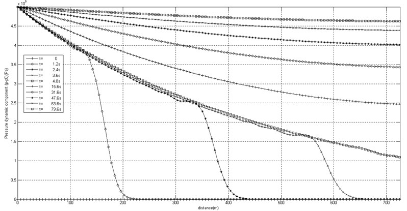
The obtained values are very similar to those obtained for the fluid with the speed of the pressure wave propagation 1112.7 m/s, as the value of bulk modulus does not bring significant changes in the coefficient of the steady flow Eq. (13). However, the wave propagation properties are obtained very different compared to previous situation. Fig. 2 illustrates the transition of the flow from one steady state to another, as the pressure pulse of 5×10⁵ Pa, duration 0.45 s is applied. Screenshots of flow mass rates distribution along the pipe at successive moments of time from 0 to 36 s are presented. After the application of the excitation pulse the input pressure acquires new steady value 4.15 MPa, and the new steady value of the flow rate should be established. Curves presented in Fig. 2(a) demonstrate how the flow rate distribution converges to the new steady value 11857 Pa (dotted line). The same value is obtained as the steady flow equation solution, as well as, as the final state of the flow transient. This verifies the validity of the dynamic finite element model. The necessity of the nodal flow mass rate balance correction is clearly demonstrated by comparing the results presented in Fig. 2(a) and Fig. 2(b). Without the correction procedure, the flow rate solution does not converge to a steady value along the pipe (Fig. 2(b)).

However, the pressure errors obtained by omitting the nodal rate balance correction are not so significant, Fig. 3. The three pictures of Fig. 3 present initial ( $t =$ 0 s) and final ( $t =$ 76 s) states of pressures, flow velocities and flow rates distribution along the pipe at three different computational options: (A) full equation system Type 3 with and without nodal rate balance correction, and (B) simplified equation system Type 1 with nodal rate balance correction. Obviously, option Type 3 with nodal rate balance correction should be considered as being closest to the exact solution. If other two options are considered, only insignificant differences of pressure values along the pipe are observed, Fig. 3(a). Velocity values at equation Type 1 are obtained erroneous at both final and initial state, because no fluid compressibility is taken into account by the equations, see Fig. 3(b). Equation Type 3 without nodal rate balance correction produces errors of flow velocities, which are quantitatively more significant than the corresponding pressure errors. The results presented in Fig. 3(c) depict the initial and final state of flow rates and should be regarded as steady flow states, to which the solutions presented in Fig. 2 converge.

As the equivalent bulk modulus of the fluid $\tilde{K}$ increases, the influence of the nodal flow rate balance correction becomes much less significant, as could be seen from the results presented in Fig. 4. It presents the initial and final state of pressures and flow mass rate at three different values of $\tilde{K} =$ 2.2×10⁷ Pa, $\tilde{K} =$ 2.2×10⁸ Pa and $\tilde{K} =$ 2.2×10⁹ Pa, which correspond to pressure wave velocity values 148.1 m/s, 452.8 m/s and 1112.7 m/s. All curves are obtained without application of the nodal rate balance correction. When the pressure wave velocity exceeds the flow velocity 10 and more times, the nodal flow rate balance is approximately held up without additional effort of correction by means of relations Eq. (20) and enables to save the computational time.

Fig. 2Superimposed screenshots of distribution of flow rate values along the pipe (pules propagation velocity 148.1 m/s) at successive moments of time in the range 0-36 s at initial steady flow velocity average value 39 m/s, EqT = 3

Superimposed screenshots of distribution of flow rate values along the pipe (pules propagation velocity 148.1 m/s) at successive moments of time in the range 0-36 s at initial steady flow velocity average value 39 m/s, EqT = 3

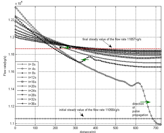
a) Nodal rate balance correction applied

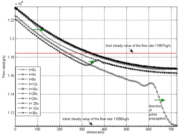
b) Without nodal rate balance correction

Fig. 3a) Steady values of pressures, b) flow velocities and c) flow rates at initial and final moments of time which are obtained after application of the pressure pulse 5×105 Pa by applying three different options of the equation system

a) Steady values of pressures, b) flow velocities and c) flow rates at initial and final moments of time which are obtained after application of the pressure pulse 5×105 Pa by applying three different options of the equation system

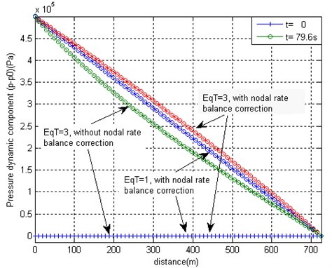
a)

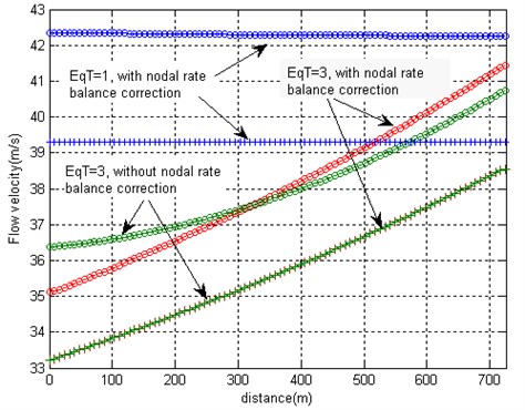
b)

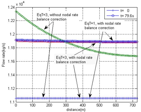
c)

Fig. 4a) Steady values of pressures and b) flow rates at the final moment of time, which are obtained after application of the pressure pulse 5×105 Pa by solving the FE model based on equation Type 3 with no nodal rate balance corrections at different values of pressure wave propagation along the pipe and steady flow velocity 39 m/s

a) Steady values of pressures and b) flow rates at the final moment of time, which are obtained after application of the pressure pulse 5×105 Pa by solving the FE model based on equation Type 3 with no nodal rate balance corrections at different values of pressure wave propagation along the pipe and steady flow velocity 39 m/s

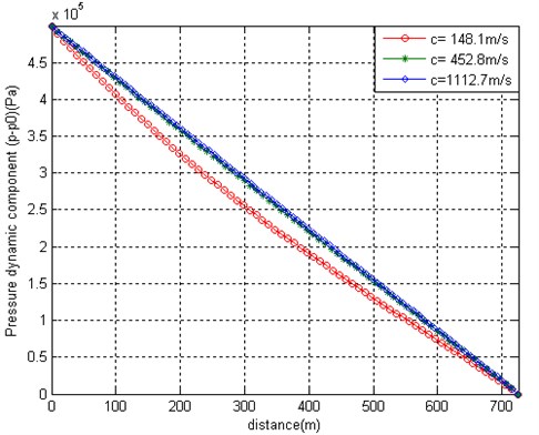
a)

b)

Fig. 5 presents the example of pressure wave propagation along the pipe, if non-reflecting boundary condition is applied at the right-hand end of the pipe. One may observe that no reflected wave is observed and the constant pressure value $p - p_{0} =$ 5×10⁵ Pa along the pipe is established in the course of time.

The presented examples verify the validity of the algorithm. In each of the presented situations the convergence of the model is observed as the computational mesh is refined.

The following example illustrates the application of the model to a real engineering situation of a pipeline, which represents a part of heating network of a city. Rather slow water flow at velocity 2-3 m/s is assumed; thus the model based on equation Type 1 could be used, and nodal rate balance correction procedure could be omitted. Only a part of pipe network has been analyzed, the prescribed pressure and non-reflecting boundary conditions being used at the cut boundaries. The initial steady flow situation was simulated by applying prescribed flow rates and reference pressure at a given point, Fig. 6.

Fig. 5Screenshots of pressure pulse propagation, where non-reflecting boundary condition is applied at the right-hand end of the pipe

The system consists of supply and return pipelines. The two parts are interconnected at numerous points, at which water consumers are connected to the pipeline. The notations used in Fig. 6 are as follows:

KPxx are key-point numbers. Pipes between each pair of key-points are of uniform diameter and wall thickness. Pipes are meshed into finite elements (not shown in the picture), the length of which depends on wave propagation speed and the duration of the excitation pressure pulse. In most cases element length 6 m was suitable for calculations;

$w = x x$ denotes the prescribed input and output steady flow rates (m³/h), positive for incoming and negative for outgoing flow. They are used for steady flow calculation, the result of which is steady pressure distribution over the pipeline. The obtained pressures serve as initial conditions for the transient analysis;

$P b = x x$ are prescribed reference pressures used for steady and transient calculation;

$P x = x x$ is the given amplitude of the pressure pulse measured with respect to the value of the pressure at steady flow situation;

NRFL are non-reflecting points corresponding to cut-off boundaries, which separate the investigated part of the pipeline from the whole pipe network. They are used for transient calculations only;

NCON are points of interconnection of supply and return pipelines, which are represented by equivalent pipes of given lengths and diameters.

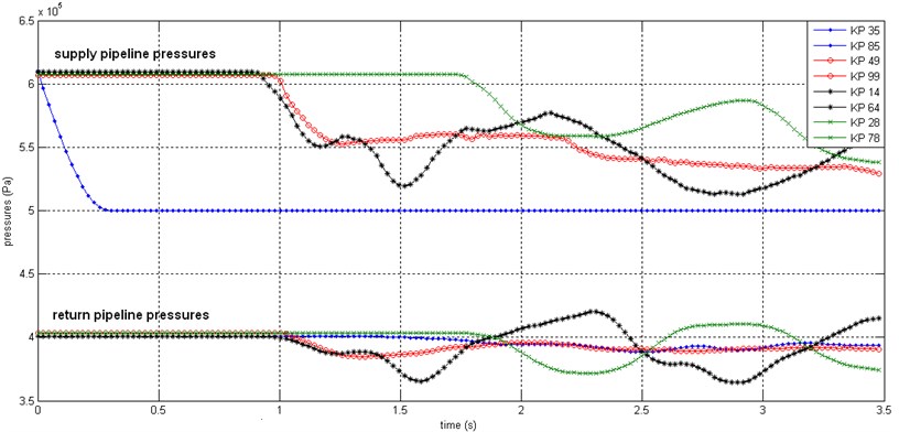
Fig. 7 presents the pressure time rates, as the pressure drops about 1×10⁵ Pa from the steady value during 0.3 s and imitates the situation of unexpected leakage in such kind of pipelines. Results of such calculations may be employed for the development of algorithms of pipeline state monitoring systems, where a change of measured pulse front shapes as the pulse propagates along the pipeline may be used for determining the locations of sudden leakages.

Fig. 6The structure of the sample pipeline – a) supply and b) return parts, which are interconnected at consumer connection points NCONxx

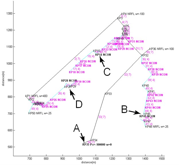
a)

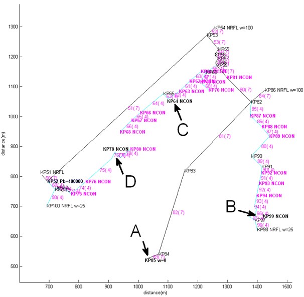
b)

Fig. 7Pressure time laws at points A, B, C and D of the supply and return parts of the pipeline presented in Fig. 6, due to the pressure drop 1e5 Pa from the steady value during 0.3 s time at KP35 (point A) of the supply pipeline imitating the situation of unexpected leakage

Pressure time laws at points A, B, C and D of the supply and return parts of the pipeline presented in Fig. 6, due to the pressure drop 1e5 Pa from the steady value during 0.3 s time at KP35 (point A) of the supply pipeline imitating the situation of unexpected leakage

5. Conclusion

The finite element scheme has been proposed for pressure wave propagation simulations in pipelines. Three analyzed options of the finite element model are based on different simplifications of the governing equation system, where the full system is one of the options. The advantage of the approach is that the pressure equation has the form of the general structural dynamic finite element equation, and the methods used for structural dynamic analysis can be directly applied to the pressure wave and vibration analysis within the pipeline. Straightforward application of the approach based on first order pressure approximation and zero order velocities approximation within finite elements can be applied only when the flow velocity is significantly less than the wave propagation velocity along the pipes. At higher flow velocities compressibility effects are taken into account, and nodal rate balance correction should be performed. Obviously, the rather expensive correction procedure is sufficient to perform every 10-20 steps. The numerical experiments demonstrate that the pressure errors are not significant even if the nodal rate balance correction is not applied, therefore considerable computational time savings could be obtained for initial estimations of the sought solution.

The possible application area of the developed model is the simulation of the pipeline leakage monitoring system, the purpose of which is to determine the location of the leakage (pressure drop pulse) basing on pressure variations registered by meters arranged at various places of the pipeline. The model can be also applied to simulations of the pressure pulse propagation in blood vessels with highly deformable walls, and in other applications.

References

Wylie E. Benjamin, Streeter Victor Lyle, Suo Lisheng Fluid Transients in Systems. Vol. 1. Prentice Hall, Englewood Cliffs, NJ, 1993.

Search CrossRef
Wood Don J., et al. Numerical methods for modeling transient flow in distribution systems. Journal of American Water Works Association, 2005, p. 104-115.

Publisher
Hwang Yao‐Hsin, ChungNien‐Mien A fast Godunov method for the water‐hammer problem. International Journal for Numerical Methods in Fluids, Vol. 40, Issue 6, 2002, p. 799-819.

Publisher
Selçuk Nevin, Tarhan Tanıl, Tanrıkulu Songül Comparison of method of lines and finite difference solutions of 2‐D Navier-Stokes equations for transient laminar pipe flow. International Journal for Numerical Methods in Engineering, Vol. 53, Issue 7, 2002, p. 1615-1628.

Publisher
Greyvenstein G. P. An implicit method for the analysis of transient flows in pipe networks. International Journal for Numerical Methods in Engineering, Vol. 53, Issue 5, 2002, p. 1127-1143.

Publisher
Frid Anders Fluid vibration in piping systems – a structural mechanics approach, I: theory. Journal of Sound and Vibration, Vol. 133, Issue 3, 1989, p. 423-438.

Publisher
Shu, Jian-Jun A finite element model and electronic analogue of pipeline pressure transients with frequency-dependent friction. Journal of Fluids Engineering, Vol. 125, Issue 1, 2003, p. 194-198.

Publisher
Kochupillai Jayaraj, Ganesan N., Padmanabhan Chandramouli A new finite element formulation based on the velocity of flow for water hammer problems. International Journal of Pressure Vessels and Piping, Vol. 82, Issue 1, 2005, p. 1-14.

Publisher
Osiadacz Andrej J. Different transient flow models-limitations, advantages, and disadvantages. PSIG Annual Meeting. Pipeline Simulation Interest Group, 1996.

Search CrossRef
Barauskas Rimantas, Barauskiene Ramute Highly convergent dynamic models obtained by modal synthesis with application to short wave pulse propagation. International Journal for Numerical Methods in Engineering, Vol. 61, Issue 14, 2004, p. 2536-2554.

Publisher
Krisciunas Andrius, Barauskas Rimantas Minimization of numerical dispersion errors in finite element models of non-homogeneous waveguides. Information and Software Technologies, Springer Berlin Heidelberg, Vol. 403, 2013, p. 357-364.

Publisher
Wolf John P., Song Chongmin Finite-Element Modelling of Unbounded Media. Wiley, Chichester, 1996.

Search CrossRef

About this article

Received

02 November 2015

Accepted

17 February 2016

Published

31 March 2016

SUBJECTS

Flow induced structural vibrations

DOI

https://doi.org/10.21595/jve.2016.16609

Keywords

finite element methods

compressible flow

dynamical systems

This is an open access article distributed under the Creative Commons Attribution License, which permits unrestricted use, distribution, and reproduction in any medium, provided the original work is properly cited.