Abstract
To solve the defects of low degradation efficiency and high cross-contamination risk in the conventional ultrasonic processor, a non-contact ultrasonic degradation system was developed. Through finite-element modal analysis, the natural frequencies of the first ten modes of the diaphragm with dome-shaped structure were found to have a ladder-like distribution, which provides a possibility to utilize the synchronous resonance of multiple modes. The effects of curvature radius, thickness and preload force on the synchronous resonance of multiple modes are studied using the control variate method, and then the structural parameters and the preload force are optimized. Based on these results, the diaphragm was manufactured, the experimental platform of the non-contact ultrasonic degradation was established, and its degradation efficiency was evaluated. The experimental results proved that the non-contact ultrasonic degradation system was able to effectively degrade Bacillus atrophaeus.
1. Introduction
Cell degradation is the premise and basis of molecular biology research; the main task of cell degradation is to break the peripheral structure of the cell, after which the target materials inside the cell (i.e., nucleic acids, enzymes, antibiotics, and etc.) are released [1]. The conventional cell degradation methods used in the laboratory include enzymatic hydrolysis [2, 3], chemical reagent degradation [4, 5] and ultrasonic degradation [6, 8]. The enzymatic hydrolysis method and the chemical reagent degradation method generally can only degrade some specific types of cells; therefore, the versatility is poorer. Moreover, the added enzyme and chemical reagents will also bring difficulty to the separation and purification of subsequent target materials. In contrast, ultrasonic degradation is a physical degradation method, having improved versatility that is suitable for diverse biological samples, with the target materials after cell degradation being prone to separation and purification.
However, the cell degradation instruments based on the ultrasonic degradation method on the market mostly are contact-type, which means the ultrasonic horn directly contacts with the sample solution to be lysed [9, 10]. The ultrasonic horn of the contact-type ultrasonic degradation processor is directly inserted into the sample solution, which brings higher risk of cross contamination. Considering the existing defects of the contact-type ultrasonic degradation instruments, this paper designs a non-contact ultrasonic degradation system based on the synchronous resonance of multiple modes, in which a diaphragm is utilized to transfer ultrasonic energy into the sample solution to avoid the direct contact of ultrasonic horn and sample solution.
2. Non-contact ultrasonic degradation system
2.1. System constituents
Non-contact ultrasonic degradation system is mainly composed of an ultrasonic excitation module, a degradation module and an auxiliary module, the schematic illustration of the system is shown in Fig. 1.
Fig. 1Schematic illustration of the non-contact ultrasonic degradation system: 1 – Ultrasonic generator, 2 – ultrasonic transducer, 3 – ultrasonic horn, 4 – diaphragm, 5 – sample solution, 6 – cell, 7 – degradation vessel, 8 – altitude adjuster, 9 – base
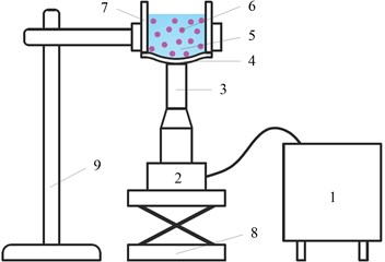
The ultrasonic excitation module is composed of an ultrasonic generator, an ultrasonic transducer and an ultrasonic horn. The ultrasonic generator converts electric supply into high-frequency AC electrical signals, which are subsequently transformed into high-frequency mechanical vibration via a transducer [11, 12].
The degradation module is a specially processed reaction container, at the bottom of which, a diaphragm made of elastic material is placed. The diaphragm is capable of vibrating at a high frequency along the longitudinal direction. A preload force should be applied between the diaphragm and the ultrasonic horn to press the ultrasonic horn against the external surface of the diaphragm tightly, as a result of which, the ultrasonic energy is able to transmit into the sample solution, causing the degradation of the cell and the release of the target material inside the cell.
Auxiliary module mainly includes a height adjuster and a base, which not only supports the whole system but also adjusts the preload force between the ultrasonic horn and the diaphragm.
2.2. Key issue
The precondition that the non-contact ultrasonic degradation system effectively disrupts the cell is that the ultrasonic wave can smoothly pass through the diaphragm and transmit into the sample solution to be lysed as much as possible. The flexural vibration performance of the diaphragm is of great importance because it directly determines the efficiency of the non-contact ultrasonic degradation system.
Ultrasonic wave is a type of longitudinal mechanical vibration whose frequency is greater than 20 kHz, and it can transmit through the medium [13, 14]. To transmit as much ultrasonic energy into the sample solution as possible, the diaphragm should resonate with the ultrasonic horn, which means the natural frequency of the diaphragm should be approximately equal to the operating frequency of the ultrasonic horn. Hence, to ensure the natural frequency of diaphragm matches the operating frequency of the ultrasonic horn, both the structure of the diaphragm and the preload force between the diaphragm and the ultrasonic horn should be optimized; this optimization is the key issue to be solved in this paper.
3. Calculation of the natural frequency of the diaphragm
3.1. Simplified model of the non-contact ultrasonic degradation system
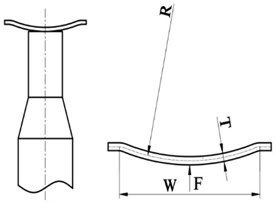
Compared with a flat diaphragm, the diaphragm with dome-shaped structure has a greater natural frequency and is apt to vibrate. The advantage of the dome-shaped design of the diaphragm is that the dome shape increases the natural frequency of the diaphragm without causing the diaphragm to be so stiff that it cannot deflect to transmit the vibratory movements and the ultrasonic energy into the sample solution. Fig. 2 is a simplified model of the non-contact ultrasonic degradation system, whose curvature radius, width and thickness are represented by , and , respectively. In addition, the preload force between the diaphragm and the ultrasonic horn is represented by .
Fig. 2Simplified model of the non-contact ultrasonic degradation system
3.2. Theoretical principle of flexural vibration
For the dome-shaped diaphragm, the differential equation of flexural vibration is given as [15]:
where , and are the mass matrix, damping matrix and stiffness matrix of the diaphragm, respectively. , and are the acceleration vector, velocity vector and displacement vector, respectively, and is the excitation force vector.
It is the physical coordinates that the equation set of motion is described by in Eq. (1). The physical coordinates of all of the mass points of the diaphragm are included in each equation, as a result of which, there is much difficulty in solving the equation set directly. Therefore, modal analysis based on the finite element method (FEM) is used to calculate the natural frequency of the diaphragm.
3.3. Finite element model of the diaphragm
The natural frequency of each mode of the diaphragm can be calculated by finite element method. Take a dome-shaped diaphragm made of acetal for example, whose structural parameters and preload force are as follows: 22 mm, 12 mm, 0.4 mm, 3 N. And the solid model of the diaphragm is designed by SolidWorks 2013, as show in Fig. 3.
Then the solid model of the diaphragm is imported into ANSYS 11.0. The element type of the diaphragm is defined as the four-noded shell element ‘SHELL63’. ‘SHELL63’ has both bending and membrane capabilities. Both in-plane and normal loads are permitted. The element has six degrees of freedom at each node, translation is allowed in all coordinate directions as well as rotation around the coordinate axes. Stress stiffening and large deflection capabilities are included.
Fig. 3Solid model of the diaphragm
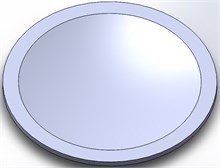
Fig. 4Finite element model of the diaphragm
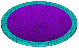
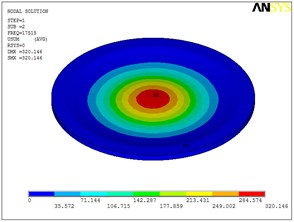
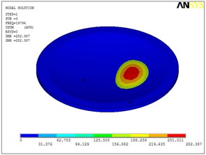
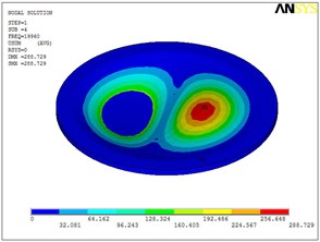
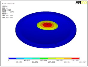
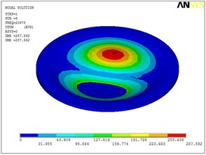
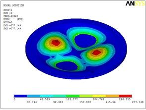
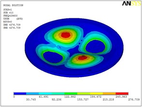
Fig. 5Eigenshapes of the first ten modes of the diaphragm
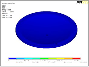
a) The first mode
b) The second mode
c) The third mode
d) The fourth mode
e) The fifth mode
f) The sixth mode
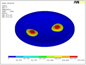
g) The seventh mode
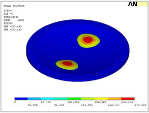
h) The eighth mode
i) The ninth mode
j) The tenth mode
In the step of meshing the model, the free meshing is used, and the size level is set to 6 by default. The finite element model, with a total of 1104 elements and 1106 nodes, is illustrated in Fig. 4. In the non-contact ultrasonic degradation system, the annular boundary part of the diaphragm is fixed on the degradation vessel, so all the DOFs of the annular boundary part’s external areas are set to be constrained.
The dome-shaped diaphragm is made of acetal, the material properties of which are shown in Table 1.
Table 1The material properties of the diaphragm made of acetal
Item | Elastic modulus (GPa) | Possion’s ratio | Density (kg/m3) |
Value | 3.378 | 0.35 | 1420 |
3.4. Natural frequencies and eigenshapes of the dome-shaped diaphragm
Based on ANSYS 11.0, static analysis of the dome-shaped diaphragm is performed, after which modal analysis is performed. Therefore, the natural frequencies and the eigenshapes of the first ten modes are extracted, as shown in Table 2 and Fig. 5.
Table 2Natural frequencies of the first ten modes (the order of the mode is represented by M1-M10)
Mode | M1 | M2 | M3 | M4 | M5 | M6 | M7 | M8 | M9 | M10 |
Natural frequency (kHz) | 17.19 | 17.52 | 19.79 | 19.96 | 20.53 | 20.68 | 28.57 | 28.66 | 29.22 | 29.60 |
3.5. Synchronous resonance of multiple modes
According to the data in Table 2, taking the order of mode as the abscissa and the natural frequency as the ordinate, the distribution of the first ten natural frequencies of the diaphragm is plotted, as shown in Fig. 6. The first ten natural frequencies of the dome-shaped diaphragm are found to have the characteristics of a ladder-like distribution. The frequencies can be divided into three gradients: the first gradient (represented by G1) is composed of M1 and M2; the second gradient (represented by G2) is composed of M3, M4, M5 and M6; and the third gradient (represented by G3) is composed of M7, M8, M9 and M10.
Fig. 6The distribution of the first ten natural frequencies of the diaphragm
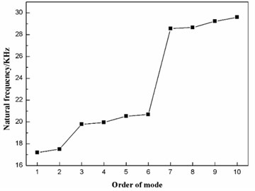
For the application of the resonance, the characteristics of the ladder-like distribution of the first ten natural frequencies of the diaphragm has the benefit to enhance the vibration intensity. When the operating frequency of the ultrasonic horn is equal to the frequency of a certain gradient (here, the frequency of gradient is defined as the mean value of the natural frequencies of the modes that are included in the gradient), the synchronous resonance of multiple modes will occur, as a result of which, the vibration intensity of the diaphragm will be enhanced.
If the operating frequency of the ultrasonic horn is equal to the frequency of the first gradient, then the diaphragm will operate in the first gradient, which means there will be only two modes (M1 and M2) violently vibrating. If the operating frequency of the ultrasonic horn is equal to the frequency of the third gradient, then the diaphragm will operate in the third gradient, and there will be four modes (M7, M8, M9 and M10). However, the frequency of the third gradient is so high that the effect of vibration damping is great. As a consequence, the second gradient should be applied to transmit as much ultrasonic energy into the sample solution as possible. Here, the operating frequency is equal to the frequency of the second gradient, and the synchronous resonance of M3, M4, M5 and M6 will occur.
4. Optimization design of the diaphragm
In the previous chapter, the vibration performance of the diaphragm having a curvature radius of 22 mm, a width of 12 mm, a thickness of 0.4 mm and a preload force of 3 N is analyzed, from which, the first ten natural frequencies are obtained, and their distribution characteristics is proposed preliminarily. To optimize the vibration performance of the diaphragm further, the factors that affect the natural frequencies of the diaphragm are analyzed in the following paragraphs.
The diaphragm to be analyzed is made of acetal having a modulus of elasticity of 3.378 GPa, a Poisson ratio of 0.35 and a density of 1420 kg/m3. It is the dimension parameter and the inner stress that affect the natural frequencies of the diaphragm. According to the design requirements of the non-contact ultrasonic degradation system, the width of the diaphragm is designed to be 12 mm, which is determined by the size of the degradation module. Therefore, the remaining factors that affect the natural frequencies of the diaphragm are the curvature radius , the thickness and the preload force .
4.1. Optimization analysis of the curvature radius
The thickness of the diaphragm and the preload force between the ultrasonic horn and the diaphragm should be kept constant when the effect of the curvature radius on the natural frequency of each mode and their distribution characteristics is analyzed. Here, the thickness is set as 0.5 mm, and the preload force is set as 0 N.
The finite element modal analysis is conducted on the diaphragm having values of the curvature radius of 15 mm, 20 mm, 25 mm, 30 mm, 35 mm and 40 mm. As a result, the natural frequencies of the first ten mode of the diaphragm with different curvature radius is obtained, as listed in Table 3. In addition, the distribution of the first ten natural frequencies of the diaphragm is plotted, as shown in Fig. 7.
Table 3The first ten natural frequencies of the diaphragm with different curvature radiuses
/ mm | Natural frequency / kHz | |||||||||
M1 | M2 | M3 | M4 | M5 | M6 | M7 | M8 | M9 | M10 | |
15 | 24.40 | 25.04 | 25.36 | 26.00 | 26.12 | 26.62 | 35.92 | 36.20 | 36.99 | 37.36 |
20 | 19.85 | 20.34 | 23.98 | 24.16 | 24.32 | 25.04 | 35.00 | 35.16 | 35.85 | 36.62 |
25 | 17.13 | 17.45 | 23.17 | 23.25 | 23.52 | 24.16 | 34.12 | 34.23 | 34.79 | 35.37 |
30 | 15.54 | 15.77 | 22.64 | 22.94 | 23.35 | 23.61 | 33.82 | 34.18 | 34.55 | 34.96 |
35 | 14.46 | 14.47 | 22.33 | 22.38 | 22.81 | 22.95 | 33.25 | 33.37 | 33.91 | 34.16 |
40 | 13.55 | 13.69 | 21.77 | 21.98 | 22.47 | 22.61 | 32.85 | 33.15 | 33.68 | 33.88 |
Fig. 7 shows that the first ten natural frequencies of the dome-shaped diaphragm with different curvature radius have characteristics of a ladder-like distribution, which is divided into three gradients: the first gradient (represented by G1) is composed of 1 and M2; the second gradient (represented by G2) is composed of M3, M4, M5 and M6; and the third gradient (represented by G3) is composed of M7, M8, M9 and M10.
According to the data in Table 3, the frequencies of the three gradients are calculated and then listed in Table 4. To evaluate the distribution characteristics of the first ten natural frequencies of the dome-shaped diaphragm with different curvature radius, an evaluation index-fluctuating frequency of gradient, is introduced. The fluctuating frequency of gradient is defined as the standard deviation of the natural frequencies of the modes that are included in the gradient. The fluctuating frequency of the gradient is capable of reflecting the deviation of the natural frequencies of the modes that are included in the gradient. Obviously, the smaller the fluctuating frequency of gradient is, the smaller the deviation of the natural frequencies is, which is more beneficial for synchronous resonance of multiple modes that are included in the gradient. According to the data in Table 3, the fluctuating frequencies of the three gradients are calculated, as listed in Table 4.
Fig. 7The distribution of the first ten natural frequencies of the diaphragm with different curvature radiuses
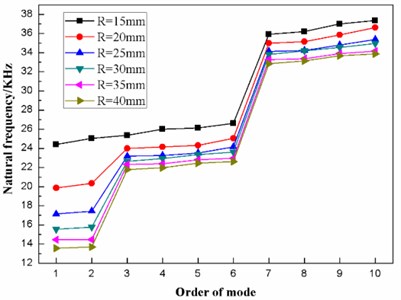
Table 4The frequencies and fluctuating frequencies of the three gradients of the diaphragm with different curvature radiuses
/ mm | Frequency of gradient / kHz | Fluctuating frequencies of gradient / kHz | ||||
G1 | G2 | G3 | G1 | G2 | G3 | |
15 | 24.72 | 26.03 | 36.62 | 0.32 | 0.45 | 0.58 |
20 | 20.10 | 24.38 | 35.66 | 0.24 | 0.40 | 0.64 |
25 | 17.29 | 23.53 | 34.63 | 0.16 | 0.39 | 0.50 |
30 | 15.66 | 23.14 | 34.38 | 0.12 | 0.37 | 0.42 |
35 | 14.47 | 22.62 | 33.67 | 0.01 | 0.27 | 0.38 |
40 | 13.62 | 22.21 | 33.39 | 0.07 | 0.34 | 0.41 |
According to Table 4, the effects of the curvature radius on the frequencies and the fluctuating frequencies of the three gradients are illustrated in Figs. 8-9, respectively.
Fig. 8Effect of the curvature radius on the frequencies of the three gradients
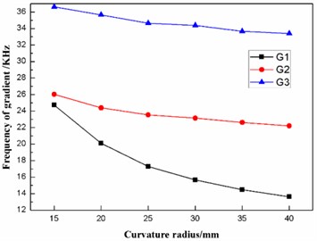
Fig. 9Effect of the curvature radius on the frequencies of the three gradients
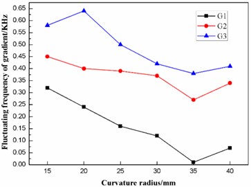
As stated in the preceding part of this paper, the diaphragm should operate in the second gradient (G2) to transmit as much ultrasonic energy into the sample solution as possible. From Figs. 8-9, it can be concluded that the frequency of the second gradient (G2) decrease gradually with the increasing curvature radius. Meanwhile, the fluctuating frequency of the second gradient (G2) reaches the minimum when the dome-shaped diaphragm has a curvature radius of 35 mm. Therefore, the curvature radius of the dome-shaped diaphragm is optimized to be 35 mm.
4.2. Optimization analysis of the thickness
The curvature radius of the diaphragm and the preload force should be kept constant when the effect of the thickness on the natural frequency of each mode and their distribution characteristics is analyzed. Here, the curvature radius is set as 35 mm, and the preload force is set as 0 N.
The finite element modal analysis is conducted on the diaphragm having values of the thickness of 0.3 mm, 0.4 mm, 0.5 mm, 0.6 mm, 0.7 mm and 0.8 mm. As a result, the natural frequencies of the first ten mode of the diaphragm with different thickness is obtained, as listed in Table 5. In addition, the distribution of the first ten natural frequencies of the diaphragm is plotted, as shown in Fig. 10.
Table 5The first ten natural frequencies of the diaphragm with different thicknesses
/ mm | Natural frequency / Hz | |||||||||
M1 | M2 | M3 | M4 | M5 | M6 | M7 | M8 | M9 | M10 | |
0.3 | 11.60 | 11.72 | 14.52 | 14.59 | 15.17 | 15.30 | 20.60 | 20.78 | 21.45 | 21.58 |
0.4 | 12.98 | 13.06 | 18.42 | 18.69 | 18.88 | 19.07 | 27.04 | 27.32 | 27.44 | 28.04 |
0.5 | 14.46 | 14.48 | 22.33 | 22.38 | 22.81 | 22.95 | 33.25 | 33.37 | 33.91 | 34.16 |
0.6 | 16.05 | 16.11 | 26.38 | 26.64 | 26.97 | 26.99 | 39.69 | 39.84 | 40.46 | 40.99 |
0.7 | 17.80 | 18.05 | 30.55 | 30.90 | 31.16 | 31.63 | 46.12 | 46.85 | 46.88 | 47.82 |
0.8 | 19.39 | 19.69 | 34.11 | 34.58 | 34.74 | 35.39 | 51.38 | 52.78 | 52.82 | 54.05 |
Fig. 10The distribution of the first ten natural frequencies of the diaphragm with different thicknesses
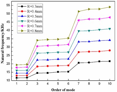
Fig. 10 shows that the first ten natural frequencies of the dome-shaped diaphragm with different thickness have characteristics of a ladder-like distribution, which is divided into three gradients: the first gradient (represented by G1) is composed of M1 and M2; the second gradient (represented by G2) is composed of M3, M4, M5 and M6; and the third gradient (represented by G3) is composed of M7, M8, M9 and M10.
According to the data in Table 5, the frequencies and the fluctuating frequencies of the three gradients are calculated, as listed in Table 6.
According to Table 6, the effects of the thickness on the frequencies and the fluctuating frequencies of the three gradients are illustrated in Figs. 11-12, respectively.
Table 6The frequencies and fluctuating frequencies of the three gradients of the diaphragm with different thickness
/ mm | Frequency of gradient / kHz | Fluctuating frequencies of gradient / kHz | ||||
G1 | G2 | G3 | G1 | G2 | G3 | |
0.3 | 11.66 | 14.90 | 21.10 | 0.06 | 0.34 | 0.42 |
0.4 | 13.02 | 18.77 | 27.46 | 0.04 | 0.24 | 0.36 |
0.5 | 14.47 | 22.62 | 33.67 | 0.01 | 0.27 | 0.38 |
0.6 | 16.08 | 26.75 | 40.25 | 0.03 | 0.25 | 0.52 |
0.7 | 17.93 | 31.06 | 46.92 | 0.13 | 0.39 | 0.60 |
0.8 | 19.54 | 34.71 | 52.76 | 0.15 | 0.46 | 0.95 |
Fig. 11Effect of the thickness on the frequencies of the three gradients
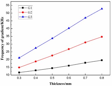
Fig. 12Effect of the thickness on the fluctuating frequencies of the three gradients
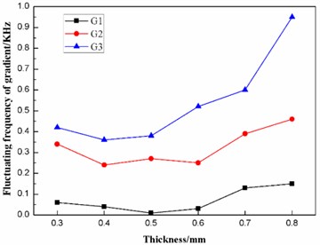
For the non-contact ultrasonic degradation system, the diaphragm should operate in the second gradient (G2) to transmit as much ultrasonic energy into the sample solution as possible, as stated above. Fig. 11 indicates that the thickness has a great effect on the frequency of the second gradient (G2). Further studies find that the frequency of the second gradient has a linear relationship with the thickness of the diaphragm. The linear-regression analysis is conducted using the least square method, and the equation of linear regression is obtained as follows:
where is the frequency of the second gradient (G2), is the thickness of the diaphragm. The square of correlation coefficient is , which proves is linearly proportional to .
The equation of linear regression has a significant reference value in engineering application. On one hand, if the thickness of the diaphragm is known, then the frequency of the second gradient can be estimated. In this case, we can choose the ultrasonic horn with a certain operating frequency to match the diaphragm. On the other hand, if the operating frequency of the ultrasonic horn has been set, then the thickness of the diaphragm can be calculated to have the frequency of the second gradient match the operating frequency of the ultrasonic horn.
It can be concluded from Fig. 12 that, when the thickness of the diaphragm is in the range of 0.4 to 0.6 mm, the fluctuating frequency of the second gradient is relatively smaller. Hence, the thickness of the diaphragm should be designed to be in the range of 0.4 to 0.6 mm.
4.3. Optimization analysis of the preload force
The curvature radius and the thickness of the diaphragm should be kept constant when the effect of the preload force on the natural frequency of each mode and their distribution characteristics is analyzed. According to the results optimized above, the curvature radius and the thickness of the diaphragm are set as 35 mm and 0.5 mm, respectively.
The finite element modal analysis is conducted on the diaphragm under values of the preload force of 0 N, 2 N, 4 N, 6 N, 8 N and 10 N. As a result, the natural frequencies of the first ten mode of the diaphragm under different preload force is obtained, as listed in Table 7. Besides, the distribution of the first ten natural frequencies of the diaphragm is plotted, as shown in Fig. 13.
Table 7The first ten natural frequencies of the diaphragm under different preload forces
/ N | Natural frequency / kHz | |||||||||
M1 | M2 | M3 | M4 | M5 | M6 | M7 | M8 | M9 | M10 | |
0 | 14.46 | 14.48 | 22.33 | 22.38 | 22.81 | 22.95 | 33.25 | 33.37 | 33.91 | 34.16 |
2 | 14.35 | 14.46 | 22.22 | 22.33 | 22.79 | 22.81 | 33.23 | 33.25 | 33.77 | 34.16 |
4 | 14.22 | 14.46 | 22.06 | 22.33 | 22.63 | 22.81 | 33.09 | 33.25 | 33.62 | 34.16 |
6 | 14.09 | 14.46 | 21.90 | 22.33 | 22.47 | 22.81 | 32.95 | 33.25 | 33.47 | 34.16 |
8 | 13.96 | 14.46 | 21.73 | 22.31 | 22.33 | 22.81 | 32.81 | 33.25 | 33.32 | 34.16 |
10 | 13.83 | 14.46 | 21.57 | 22.14 | 22.33 | 22.81 | 32.67 | 33.17 | 33.25 | 34.16 |
Fig. 13The distribution of the first ten natural frequencies of the diaphragm under different preload forces
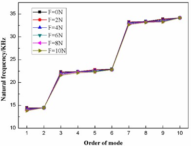
From Table 7, when the preload force ranges between 0 N and 10 N, the frequency of each mode changes little, as a result of which, the six distribution curves in Fig. 13 are interlaced with each other. However, it is clear that the first ten natural frequencies of the dome-shaped diaphragm under different preload forces have characteristics of a ladder-like distribution, which can be divided into three gradients: the first gradient (represented by G1) is composed of M1 and M2; the second gradient (represented by G2) is composed of M3, M4, M5 and M6; and the third gradient (represented by G3) is composed of M7, M8, M9 and M10.
According to Table 7, the frequencies and the fluctuating frequencies of the three gradients are calculated, as listed in Table 8.
Table 8The frequencies and fluctuating frequencies of the three gradients of the diaphragm under different preload forces
/ N | Frequency of gradient / kHz | Fluctuating frequencies of gradient / kHz | ||||
G1 | G2 | G3 | G1 | G2 | G3 | |
0 | 14.47 | 22.62 | 33.67 | 0.01 | 0.27 | 0.38 |
2 | 14.41 | 22.54 | 33.60 | 0.06 | 0.27 | 0.39 |
4 | 14.34 | 22.46 | 33.53 | 0.12 | 0.29 | 0.41 |
6 | 14.28 | 22.38 | 33.46 | 0.19 | 0.33 | 0.45 |
8 | 14.21 | 22.30 | 33.39 | 0.25 | 0.38 | 0.49 |
10 | 14.15 | 22.21 | 33.31 | 0.32 | 0.44 | 0.54 |
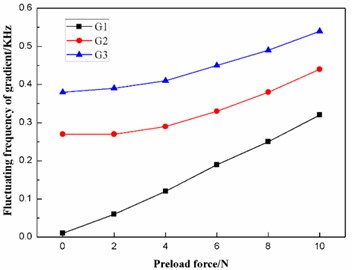
According to Table 8, the effects of the preload force on the frequencies and the fluctuating frequencies of the three gradients are illustrated in Figs. 14-15, respectively.
Fig. 14Effect of the preload force on the frequencies of the three gradients
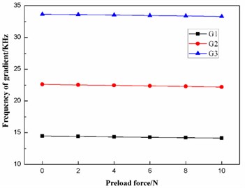
Fig. 15Effect of the preload force on the fluctuating frequencies of the three gradients
The diaphragm should operate in the second gradient (G2), as stated above. It can be concluded from Fig. 14 that the preload force has a slight effect on the frequency of the second gradient (G2). Further studies indicate that the frequency of the second gradient has a linear relationship with the preload force between the diaphragm and the ultrasonic horn. The linear-regression analysis is conducted using the least square method, and the equation of linear regression is obtained as follows:
where is the frequency of the second gradient (G2), and is the preload force between the diaphragm and the ultrasonic horn. The square of the correlation coefficient is , which proves is linearly dependent on .
The equation of linear regression also has a significant reference value in engineering application. If the structure of the diaphragm has been set, that is, the curvature radius and the thickness of the diaphragm have both been set, then the frequency of the second gradient can be fine-tuned to match the operating frequency of the ultrasonic horn through changing the value of the preload force .
5. Evaluation of the non-contact ultrasonic degradation system
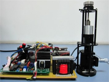
Based on the optimized results above, the dome-shaped diaphragm having a width of 12 mm, a curvature radius of 35 mm and a thickness of 0.5 mm was manufactured. The operating frequency of the ultrasonic horn is set as 22.5 kHz. It can be deduced from Eq. (3) that a preload force of 3 N should be applied between the diaphragm and the ultrasonic horn. Next, the experimental platform of the non-contact ultrasonic degradation system is established, as illustrated in Fig. 16.
Fig. 16The experimental platform
Bacillus atrophaeus (ATCC 9372) is chosen as sample to be lysed by the experimental platform because it is usually difficult to lyse bacillus atrophaeus using conventional methods in the laboratory. The degradation efficiency is calculated through plate cultivation, and then a comparison is made between the experimental platform and Branson Sonifier® S-250D digital ultrasonic processor (a contact ultrasonic degradation instrument).
5.1. Experimental methods
The concentration of the raw sample solution of bacillus atrophaeus is 106 cfu/mL. Then take 1500 µL and divide them into three parts on average, which are marked as Group A, B and C. That is to say the volume of each group is 500 µL. The main experimental procedure is illustrated in Fig. 17.
Fig. 17The main experimental procedure

1) Group A is degraded by the non-contact ultrasonic degradation system.
Group A is degraded by the experimental platform of the non-contact ultrasonic degradation system for 60 seconds. It’s impossible to count the amount of the bacillus atrophaeus that have been degraded by the experimental platform, while the amount of the bacillus atrophaeus that remain alive can be counted through plate cultivation. After degradation, the amount of bacillus atrophaeus that remain alive is represented by , here ‘1’ means the sample solution after degradation is not diluted, ‘500’ means the volume of the sample solution is 500 µL.
cannot be obtained directly since there will be loss in volume after degradation. So 100 µL of the sample solution after degradation is taken to do the following experiments. And the amount of acillus atrophaeus that remain alive is represented by . Therefore, the relation between and is as follows:
However, cannot be obtained directly through plate cultivation since the value of is too huge to count after plate cultivation, which means dilution is a necessary step before plate cultivation. So the 100 µL of the sample solution after degradation is diluted, the dilution factor of which is 1:100. After dilution, take 150 µL and divided them into three parts on average, namely the volume of each part is 50 µL. Then three parts are inoculated on three agar plates independently, which are placed into the incubator at a temperature of 36 °C and then inverted. 24 hours later, the three agar plates are taken from the incubator, and then the colonies of bacillus atrophaeus are counted. The amount of bacillus atrophaeus in each agar plate is represented by , and , and the mean value of , and is represented by . Here ‘100’ means the dilution factor is 1:100, and ‘50’ means the volume of bacillus atrophaeus solution inoculated on agar plate is 50 µL. Therefore, the relation between and is as follows:
2) Group B is degraded by the conventional ultrasonic processor.
Group B is degraded by Branson Sonifier® S-250D digital ultrasonic processor for 60 seconds. After degradation, the amount of bacillus atrophaeus that remain alive is represented by , here ‘1’ means the sample solution after degradation is not diluted, ‘500’ means the volume of the sample solution is 500 µL.
cannot be obtained directly. So 100 µL of the sample solution after degradation is taken to do the following experiments. And the amount of acillus atrophaeus that remain alive is represented by . Therefore, the relation between and is as follows:
cannot be obtained directly through plate cultivation, and dilution is a necessary step before plate cultivation. So the 100 µL of the sample solution after degradation is diluted, the dilution factor of which is 1:100. After dilution, take 150 µL and divided them into three parts on average, namely the volume of each part is 50 µL. The three parts are inoculated on three agar plates independently, which are placed into the incubator at a temperature of 36 °C and then inverted. 24 hours later, the three agar plates are taken from the incubator, and then the colonies of bacillus atrophaeus are counted. The amount of bacillus atrophaeus in each agar plate is represented by , and , and the mean value of , and is represented by . Here ‘100’ means the dilution factor is 1:100, and ‘50’ means the volume of bacillus atrophaeus solution inoculated on agar plate is 50 µL. Therefore, the relation between and is as follows:
3) Group C is not degraded.
Group C is not degraded, and the amount of bacillus atrophaeus in group C is represented by . Here ‘1’ means group C is not diluted, ‘500’ means the volume of group C is 500 µL. Obviously, can be regarded as the amount of bacillus atrophaeus in group A or B before degradation.
Take 100 µL from group C, the amount of bacillus atrophaeus in it is represented by . The relation between and is as follows:
However, cannot be obtained directly through plate cultivation, and dilution is a necessary step before plate cultivation. This time the dilution factor is 1:1000 because the value of is huger. After dilution, take 150 µL and divided them into three parts on average, namely the volume of each part is 50 µL. The three parts are inoculated on three agar plates independently, which are placed into the incubator at a temperature of 36 °C and then inverted. 24 hours later, the three agar plates are taken from the incubator, and then the colonies of bacillus atrophaeus are counted. The amount of bacillus atrophaeus in each agar plate is represented by , and , and the mean value of , and is represented by . Here ‘1000’ means the dilution factor is 1:1000, and ‘50’ means the volume of bacillus atrophaeus solution inoculated on agar plate is 50 µL. Therefore, the relation between and is as follows:
4) Calculation of the degradation efficiency.
The degradation efficiency is defined as the ratio of the amount of the bacillus atrophaeus that has been degraded to the total amount of the bacillus atrophaeus without any treatment and is represented by . Therefore, the degradation efficiencies of the experimental platform and the Branson Sonifier® S-250D digital ultrasonic processor are as follows:
According to Eqs. (4)-(12), the degradation efficiencies can be given as:
5.2. Experimental results
The results are listed in Tables 9-11, from which the degradation efficiency can be calculated.
86.7 %, 82.5 %.
The results prove that the non-contact ultrasonic degradation system developed in this paper has the ability to degrade bacillus atrophaeus.
Table 9The amount of bacillus atrophaeus from Group A (after cultivation)
313 | 330 | 272 | 305 |
Table 10The amount of bacillus atrophaeus from Group B (after cultivation)
425 | 382 | 398 | 401.7 |
Table 11The amount of bacillus atrophaeus from Group C (after cultivation)
244 | 225 | 219 | 229.3 |
6. Conclusions
1) Using a diaphragm, the non-contact ultrasonic degradation system developed in this paper can avoid the high risk of cross contamination that plagues conventional ultrasonic processors.
2) Based on the finite element modal analysis, the first ten natural frequencies of the dome-shaped diaphragm are found to have the characteristics of a ladder-like distribution, which provides a possibility to utilize the synchronous resonance of multiple modes.
3) To optimize the vibration performance of the diaphragm, the effects of the curvature radius, the thickness and the preload force on the frequency and the fluctuating frequency of the second gradient are analyzed. In addition, some laws of significant reference value are discovered.
4) According to the optimized results, the dome-shaped diaphragm is manufactured and the experimental platform is established, through which the experiments are conducted. The results prove that non-contact ultrasonic degradation system developed in this paper is capable of effectively degrading bacillus atrophaeus.
References
-
Kowalczyk M., Kolakowski P., Bienkowska J. M. R., Szmytkowska A., Bardowski J. Cascade cell lyses and DNA extraction for identification of genes and microorganisms in kefir grains. Journal of Dairy Research, Vol. 79, Issue 1, 2012, p. 26-32.
-
Ensign J., Wolfe R. S. Characterization of a small proteolytic enzyme which lyses bacterial cell walls. Journal of Bacteriology, Vol. 91, Issue 2, 1966, p. 524-534.
-
Salazar O., Asenjo J. A. Enzymatic lysis of microbial cells. Biotechnology Letters, Vol. 29, Issue 7, 2007, p. 985-994.
-
Novella S., Fargues C., Grevillot G. Improvement of the extraction of penicillin acylase from Escherichia coli cells by a combined use of chemical methods. Biotechnology and Bioengineering, Vol. 44, Issue 3, 1994, p. 379-382.
-
Falconer R. J., Neill B. K., Middelberg A. P. J. Chemical treatment of escherichia coli: extraction of intracellular protein from uninduced cells. Biotechnology and Bioengineering, Vol. 53, Issue 3, 1997, p. 453-458.
-
Taylor M. T., Belgrader P., Furman B. J. Lysing bacterial spores by sonication through a flexible interface in a microfluidic system. Analytical Chemistry, Vol. 73, Issue 3, 2001, p. 492-496.
-
Fykse E. M., Olsen J. S., Skogan G. Application of sonication to release DNA from Bacillus cereus for quantitative detection by real-time PCR. Journal of Microbiological Methods, Vol. 55, Issue 1, 2003, p. 1-10.
-
Marentis T. C., Kusler B., Yaralioglu G. G. Microfluidic sonicator for real-time disruption of eukaryotic cells and bacterial spores for DNA analysis. Ultrasound in Medicine and Biology, Vol. 31, Issue 9, 2005, p. 1265-1277.
-
Skauen D. A. Comparison of heat production and cavitational intensity in several ultrasonic cell disruptors. Ultrasonics, Vol. 14, Issue 4, 1976, p. 173-176.
-
Barros W. R. P., Steter J. R., Lanza M. R. V., Motheo A. J. Degradation of amaranth dye in alkaline medium by ultrasonic cavitation coupled with electrochemical oxidation using a boron-doped diamond anode. Electrochimica Acta, Vol. 143, Issue 10, 2014, p. 180-187.
-
Liu H. L., Hua M. Y., Chen P. Y. Blood-brain barrier disruption with focused ultrasound enhances delivery of chemotherapeutic drugs for glioblastoma treatment. Radiology, Vol. 255, Issue 2, 2010, p. 415-425.
-
Newcomb W. L., Hope W. W., Schmelzer T. M. Comparison of blood vessel sealing among new electrosurgical and ultrasonic devices. Surgical Endoscopy, Vol. 23, Issue 1, 2009, p. 90-96.
-
Harb M. S., Yuan F. G. A rapid, fully non-contact, hybrid system for generating Lamb wave dispersion curves. Ultrasonics, Vol. 61, 2015, p. 62-70.
-
Deng M. X., Xiang Y. X. Analysis of second-harmonic generation by primary ultrasonic guided wave propagation in a piezoelectric plate. Ultrasonics, Vol. 61, 2015, p. 121-125.
-
Lin S. Y. Study on the flexural vibration of rectangular thin plates with free boundary conditions. Journal of Sound and Vibration, Vol. 239, Issue 5, 2001, p. 1063-1071.
About this article

Longxue Qiao developed the non-contact ultrasonic degradation system and wrote the manuscript. Yaohua Du optimized the structural parameters of the dome-shaped diaphragm as well as the preload force. Feng Chen designed the experiments to evaluate the system. Jinlong Wu performed the experiments and analyzed the data. Taihu Wu provided instruction and financial supports.
