Design on the fairwater shape and its influence on the radiation noise of submarines

Huo, Lin; Fei, Si-miao

doi:10.21595/jve.2016.16942

Journal of Vibroengineering

Browse Journal

Submit article

Published: 31 December 2016

Check for updates

Design on the fairwater shape and its influence on the radiation noise of submarines

Lin Huo¹

Si-miao Fei²

¹School of Safety Engineering, Shenyang Aerospace University, Shenyang, 110000, China

²Shenyang Aircraft Design and Research Institute, Shenyang, 110000, China

Corresponding Author:

Lin Huo

Cite the article Download PDF

Downloads 1618

WoS Core Citations 1

CrossRef Citations 1

Abstract

Firstly, a numerical computation model of submarine radiation noise was established to obtain the radiation noise of the submarine, which was compared with the experimental results, thus verifying the validity of the model. As indicated by the computational result, the submarine fairwater played a significant impact on radiation noise at the front section, whose structure was therefore necessary to be studied. In the paper, there were several different type submarine fairwaters. Large eddy simulation (LES) and boundary element method (BEM) were applied to conduct the numerical computation for the vortex flow field and acoustic characteristics of the original fairwater, the fairwater with fillet and the streamline fairwater. Furthermore, the impact and suppression effect of the fairwater’s type on wall pressure fluctuations and flow-induced noise were analyzed. As shown from the research, the vertical fairwater with fillet or the streamline fairwater can significantly improve the flow quality, thus considerably reducing the pressure fluctuations and flow-induced noise. The paper is conductive to the academic research of flow noise of submarine as well as the new submarine design in the future.

1. Introduction

As one of three major noise sources of a submarine, flow noises cannot be reduced by the method used for mechanical noises. The submarine cover was directly exposed in the fluid and a fairwater caused turbulent flows on the submarine surface, so that strong fluctuating pressure can be generated, acted on the submarine surface and directly radiated noises. Flow noise intensity rapidly increased with the increase of the speed, while the radiated sound power was in proportion to 5th-7th power of the speed [1]. Submarine designers have paid more and more attention to the importance of flow noises.

Current researches on flow noises were mainly completed through experimental measurement and numerical simulation [2, 3]. Martin [4] has adopted a self-propelled model experiment to obtain time-domain signals of submarine flow noises combining with an effective signal processing method. Reference [5] applied the computational fluid dynamic software and computed the submarine fairwater position and fluctuating pressure intensity. Skudrzyk [6] applied hydrophones with different dimensions to carry out noise measurement of the revolution, analyzed influences brought by hydrophones with different dimensions on measurement results, wrapped materials with different roughness on the surface of revolution solid to analyze their influences on the results. Lu [7] applied FLUENT software to carry out numerical simulation of flow noises of the submarine by loading different appendages and analyzed influences brought by different appendages on noises. Zeng [8] predicted flow noises of a submarine with full appendages by combining computational fluid mechanics and boundary element method and analyzed the changing regulation of acoustic directivity under different frequencies, where the computational results were consistent with general acoustic regulations. The mentioned researches computed flow noises only through experiments or numerical simulation. And they aimed at a certain submarine model, but failed to research the submarine fairwater.

The paper computed the flow field on submarine surface based on large eddy simulation firstly, and then applied the boundary element method to compute flow noises and radiation noises on the submarine surface. The submarine fairwater was changed into two different structures, while their flow noises were computed respectively for comparative analysis.

2. Numerical simulation method

2.1. Equation of large eddy simulation

Continuity equation and NS equation of filtering waves can be expressed as follows:

1

\frac{\partial ρ}{\partial t} + \frac{\partial}{\partial x_{i}} (ρ {\bar{u}}_{i}) = 0,

2

\frac{\partial}{\partial t} (ρ {\bar{u}}_{i}) + \frac{\partial}{\partial x_{j}} (ρ {\bar{u}}_{i} {\bar{u}}_{j}) = \frac{\partial}{\partial x_{j}} (μ \frac{\partial σ_{i j}}{\partial x_{j}}) - \frac{\partial \bar{p}}{\partial x_{i}} - \frac{\partial τ_{i j}}{\partial x_{j}} .

Wherein: $σ_{i j}$ was the stress tensor caused by molecular viscosity, and $τ_{i j}$ was the subgrid stress. Subgrid eddy simulation model is used for simulation:

3

σ_{i j} = [μ (\frac{\partial {\bar{u}}_{i}}{\partial x_{j}} + \frac{\partial {\bar{u}}_{j}}{\partial x_{i}})] - \frac{2}{3} μ \frac{\partial {\bar{u}}_{i}}{\partial x_{i}} δ_{i j},

4

τ_{i j} = ρ \bar{u_{i} u_{j}} - ρ {\bar{u}}_{i} {\bar{u}}_{j} .

If ${u'}_{j} = u_{j} - {\bar{u}}_{j}$ was a small-scale movement, $τ_{i j}$ can be divided into the following formula:

5

τ_{i j} = (\bar{{\bar{u}}_{i} {\bar{u}}_{j}} - {\bar{u}}_{i} {\bar{u}}_{j}) + (\bar{{\bar{u}}_{i} {u'}_{j}} + \bar{{u'}_{i}_{i} {\bar{u}}_{j}}) + \bar{{u'}_{i} {u'}_{j}} .

Wherein: the first term was called Leonard term, also known as out scatter term, which represented the interaction between two large eddies to produce small-scale turbulence; the second of cross term meant the interaction between large and small eddies, whose energy can be transferred from large eddy to small one, vice versa, but the energy was transmitted from large eddy to the small one generally; the third of backscatter term demonstrated the large eddy generated from the interaction between two small eddies, whose energy was transferred from small eddy to large one. It was believed previously that different models should be applied to approximate various terms due to their distinct physical meanings. However, owing to the imperfect modeling technology yet, respective modeling may not be accurate and thus meaningless. Therefore, they tended to assemble together to conduct the overall modeling.

Dynamic Smagorinsky model was applied in the paper to simulate subgrid stress. Proposed by Germano in 1991, the model tried to reflect the actual flow by calculating eddy viscosity coefficient dynamically. Information of the minimum solvable scale was sampled, and then it was applied to simulate the subgrid scale stress. Near the boundary of the wall, the model gave correct asymptotic properties, which did not require damping function or intermittent function. The impact of backscatter was also considered in the model. And Lilly (1992) improved it through the least square method. Please refer to literature for detailed formula derivation and meaning.

2.2. Equation of acoustic analogy

Ffowcs Williams and Hawkins acoustic analogy equation, namely FW-H equation, was expressed as follows:

6

\frac{1}{c_{0}^{2}} \frac{\partial^{2} p^{'}}{\partial t^{2}} - \nabla^{2} p^{'} = \frac{\partial^{2}}{\partial x_{i} \partial x_{j}} [T_{i j} H (f)] - \frac{\partial}{\partial x_{i}} \{[P_{i j} n_{j} + ρ u_{i} (u_{n} - υ_{n})] δ (f)\}

+ \frac{\partial}{\partial t} \{[ρ_{0} υ_{n} + ρ υ_{i} (u_{n} - υ_{n})] δ (f)\} .

Wherein: $u_{i}$ was the fluid velocity component in $x_{i}$ direction; $u_{n}$ represented the fluid velocity component perpendicular to the object surface ( $f =$ 0); $υ_{i}$ expressed the velocity component of object surface in $x_{i}$ direction; $υ_{n}$ was the normal velocity component of object surface; $δ (f)$ meant the Dirac delta function; and $H (f)$ indicated the Heaviside step function. $p'$ meant the far-field sound pressure. $f =$ 0 indicated the object surface, and $f >$ 0 represented the externally unbounded free space. $n_{j}$ expressed the exterior normal of object surface, pointing at the inside fluid. $c_{0}$ was the far-field sound velocity, $ρ_{0}$ indicated the far-field density, and $T_{i j}$ expressed the Lighthill stress tensor.

7

T_{i j} = ρ u_{i} u_{j} + [(p - p_{0}) - c_{0}^{2} (ρ - ρ_{0})] δ_{i j} - τ_{i j} .

The far-field solution could be obtained through free-space Green function $δ (g) / 4 π r$ . The combination method of Kirchhoff integral and seepage FW-H method that was permeable through a surface was actually applied in the paper. And the far-field sound was consisted of monopole noise ${p'}_{T} (x, t)$ , dipole noise ${p'}_{L} (x, t)$ and quadrupole noise ${p'}_{Q} (x, t)$ .

8

p^{'} (x, t) = {p^{'}}_{T} (x, t) + {p^{'}}_{L} (x, t) + {p^{'}}_{Q} (x, t) .

2.3. Computational characteristic of flow-induced noise

Crighton [9] pointed out that the computation of flow-induced noise was faced with more challenges compared to general problems. And this issue is given detailed discussion by Colonius and Lele [10] in recent years.

Firstly, the steady computation method cannot be used since the flow generating noise must be unsteady. However, unsteady RANS method was difficult to achieve sufficient computational requirements. Therefore, modern turbulence simulation technologies such as DNS, LES and DES should be applied to simulate unsteady flow noises. Nevertheless, their computational costs were huge, which was generally conducted on a high-performance parallel computer. Both LES and DES included simulations and approximations for different scales of flows. And the impact of this treatment on flow noise prediction was a problem with fairly theoretical depth, which cannot be thoroughly inspected and interpreted so far.

Second, an enormous difference was presented in the disturbance amplitude and characteristic scale of fluid mechanics and acoustics. Except high-speed flow containing shock wave and other few cases, only a small portion of fluid can be converted to acoustic energy in the far field. In the direct method (CAA), the sound and flow were solved simultaneously, which had very strict requirements for the form of numerical difference. In the combination approach (CFD+acoustic analogy), the sound and flow were calculated separately, the numerical precision also needed to be achieved a reasonable level, and the expression of the used sound source must be faithful to its actual radiation characteristics.

The outstanding problem existing in the flow acoustics was the scale separation of flow and sound, which brought not only computational challenges, but computational simplification. Its key was depended on the selected methods of the investigator. In infinite region, acoustic waves and hydrodynamic sources were matched in terms of time scale, and its wavelength $λ$ and the source (vortex) scale $l$ were approximately expressed as $λ = l / M$ through the Mach number $M$ . In the flow with low Match number, namely $M$ << 1, a huge difference between l and $λ$ was thus generated, thereby causing the direct calculation of sound change to be very difficult. On the other hand, a huge difference on the scale enabled the combination method to be reasonable, simple and practical. That is to say, if the sound energy was too small to produce an effective impact on the fluid motion, the flow information can be calculated firstly and then substituted into the acoustic equation to solve the sound.

2.4. Computational results of the flow field

The model of submarine was shown in Fig. 1, and its boundary conditions in the computational process of flow characteristic were as follows.

Speed inlet: 2L forwards of the submarine head. The magnitude and direction of the inflow velocity were set.

Pressure outlet: 4L backwards of the submarine tail. The hydrostatic pressure value of the flow was set corresponding to the reference point.

Wall: Outer surface of the submarine. Suppose there is no slip adhesion condition.

Far field: 2L away from the submarine surface, whose speed was the speed of the undisturbed mainstream zone.

Wherein: L refers to the length of the submarine.

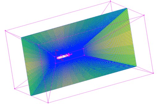
According to above boundary conditions, the computational model of submarine flow field could be obtained, as shown in Fig. 2. Both structured meshes and unstructured meshes, with the total number of 1.4 million, were included in the model, so as to achieve better computational accuracy. The computational steps were as follows: an inflow velocity was given firstly, the steady computation was conducted till its sufficient convergence, and then the accuracy of the flow field simulation was verified. Under a relatively satisfactory accuracy, this steady solution was taken as the initial value for unsteady computation. The time step of 0.00005 s was selected for unsteady computation, so as to capture the characteristics at high frequency.

Fig. 1Geometric model size of submarines

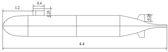
Fig. 2Computational model of submarine flow field

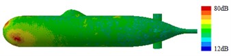
Based on the above computational model, distribution of surface pressure and vorticity of submarines could be obtained, as shown in Fig. 3. It was shown in Fig. 3 that pressure and vorticity were distributed extensively at the head section and appendages of the submarine. The head section was an initial position which could generate interactions with a fluid, so a large pressure difference could be formed on the surface. Due to sudden structure changes in the appendages, serious separated vortexes would be generated on the surface, so that large pressure could be caused.

Fig. 3Computational results of flow field on submarine surface

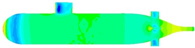
a) Pressure distribution

b) Vorticity distribution

3. Verification of numerical computation model

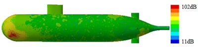
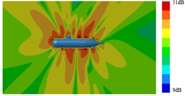
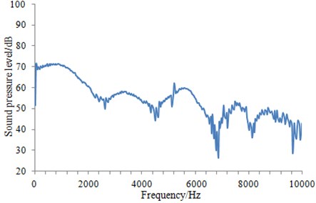
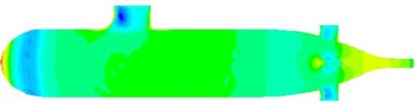
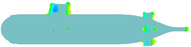
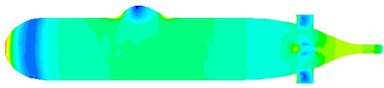
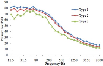
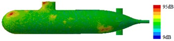
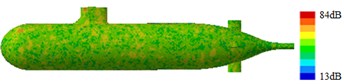
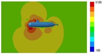
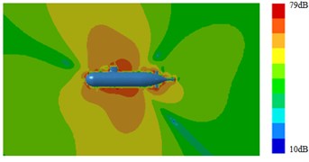
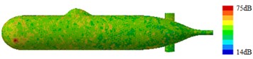
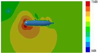
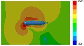
Outer surface of the geometric model was extracted to be meshed, as shown in Fig. 4. The model mainly adopted triangular elements. There were 10981 elements and 12153 nodes in total. The computational elastic material modulus was 2.1e11, density was 7800 kg/m³ and Poisson's ratio was 0.31. Then, Fig. 4 which was coupled with the flow field characteristics computed in Fig. 3 was imported into VIRTUAL.LAB. The boundary element meshes and structural meshes were coupled to map all flow field characteristics onto the boundary element mesh. Hence, all features of structural meshes can be obtained by the boundary element mesh. Then, the sound field was computed, as shown in Fig. 5 and Fig. 6. It was shown in Fig. 5 that with increase of the analyzed frequency, the noise on submarine surface decreased gradually. When the analyzed frequency was 100 Hz, noises on the submarine surface were mainly distributed around the head section, and noises of other positions were relatively uniform. With increase of the analyzed frequency, noise distribution on the submarine surface became uniform gradually. It was shown in Fig. 6 that, when the analyzed frequency was 100 Hz, the radiation noise of submarines mainly came from the head section. When the analyzed frequency was 500 Hz, the radiation noise of submarines was mainly caused by appendages on the submarine surface. When the analyzed frequency kept on increasing, the radiation noise of submarines presented obvious directivity. The spectral response of pressure at 1.0 m ahead of submarine was extracted as shown in Fig. 7. It was indicated that more peaks and valleys were appeared in the sound pressure response. However, it was gradually decreased with the increasing frequency on the overall trend.

Fig. 4Boundary element meshes of submarine

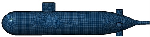
Fig. 5Contours of sound pressures of submarine surfaces

a) 100 Hz

b) 1000 Hz

c) 2000 Hz

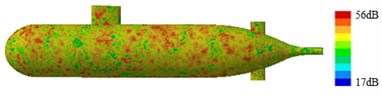
d) 5000 Hz

Fig. 6Contours of radiation noises of submarines

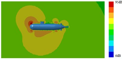
a) 100 Hz

b) 1000 Hz

c) 2000 Hz

d) 5000 Hz

Fig. 7Field point SPL at the head section of the submarine

Concerning the submarine, its radiation noise had the very complex numerical computation, whose validation through tests was necessary to be conducted for better computational precision.

Fig. 8Experimental process of the submarine radiation noise

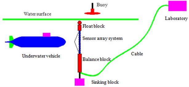
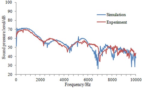
The shallow sea was selected in the paper, as shown in Fig. 8, so as to check the radiation noise regarding submarine. On the water surface, a buoy was placed so that the submarine can drive safely; and a sensor array system was arranged in the middle of floating sinking blocks under water. Additionally, a balance block was installed between the sinking block and the sensor array system, so as to confirm the stability of the latter under extrinsic factors. We connected the cable to the laboratory, and carried out the experiment later. To coincide with the numerical simulation process greatly, the experiment was set with the time step of 10 s, which was carried out for 3 times. Their mean value was selected as the final test value, which was compared with that of the numerical value in the simulation as Fig. 9. As seen from Fig. 9, experiment and simulation were basically consistent in terms of both values and trends, thus indicating the computational model reliability of the sound field established in this paper, which can be effectively used for subsequent analysis.

Fig. 9Comparison of experiment and simulation for sound pressure

4. Suppression on submarine radiation noises

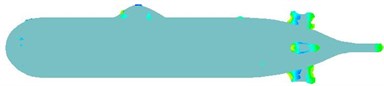
As seen from Fig. 5 and Fig. 6, the fairwater played a greater impact on sound field response of the submarine surface, whose structure was therefore necessary to be studied. Firstly, a fairwater with fillet at front edge and a streamline fairwater were designed, so as to weaken vortex at the connection section and suppress pressure fluctuations by these measures. Next, the verified LES method was applied to compute the vortex field of three types of fairwaters. Meanwhile, the impact of three types of fairwaters on wall pressure fluctuations and flow-induced noise was also analyzed. Three models were shown in Fig. 10, and 8 sampling points were located on the fairwater. Sampling points on the fairwater were basically same corresponding to the main body, and the changes of their pressure fluctuations were comparable.

Fig. 10Geometric models of three kinds of submarines

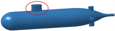
a) Type 1

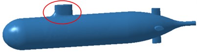
b) Type 2

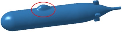
c) Type 3

4.1. Flow fields of different fairwaters

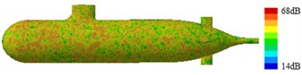
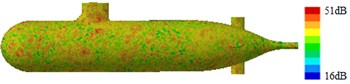
The computational results of the flow filed were shown as Fig. 11 and Fig. 12. It was shown in comparison between Fig. 3 and Fig. 11 that pressure distribution and vorticity distribution of two structures were highly similar, while there was no obvious change basically. However, it was shown in comparison between Fig. 3 and Fig. 12 that pressure distribution and vorticity distribution of the submarine surface changed very obviously. There was basically no vortex on the fairwater of Type 3 submarine, while pressures at the head and middle parts were also improved to a certain extent.

Fig. 11Computational results of flow field on surface of type 2 submarine

a) Pressure distribution

b) Vorticity distribution

Fig. 12Computational results of flow field on surface of type 3 submarine

a) Pressure distribution

b) Vorticity distribution

4.2. Pressure fluctuations of different observation points for fairwaters

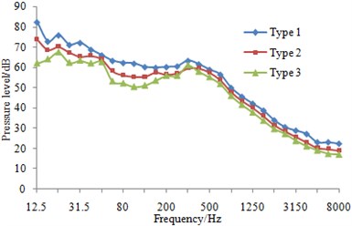
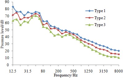
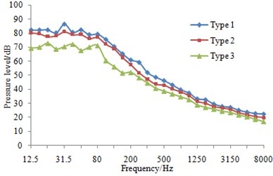
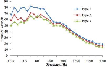
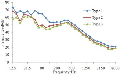
At eight sampling points on the surface of three types of fairwaters, the 1/3 octave result of pressure fluctuations can be found in Fig. 13. It could be known that compared with the original proposal, the fairwater with fillet and the streamline fairwater were declined to different degrees in terms of spectral amplitude of the pressure fluctuations. Furthermore, points P1 and P5 were reduced maximally, and low-frequency band was shown more significant reduction amplitude than the high-frequency band. Regarding fairwater with fillet, pressure fluctuations of point P1 was reduced 1~25.1 dB, point P2 was reduced by 1~11.5 dB, P3 was reduced by 1~12.4 dB, P4 was reduced by 1~8.8 dB, P5 was reduced by 1~31.5 dB, P6 was reduced by 1~18.1 dB, P7 was reduced by 2~24.4 dB, and P8 was reduced by 1~3.8 dB. Regarding the streamline fairwater, pressure fluctuations of point P1 was reduced by 1~27.1 dB, P2 was reduced by 1~19.1 dB, P3 was reduced by 1~21.6 dB, P4 was reduced by 2~18.7 dB, P5 was reduced by 2~31.8 dB, P6 was reduced by 1~14.8 dB, P7 was reduced by 5~25.9 dB, and P8 was reduced by 1~27.8 dB.

The total sound level of pressure fluctuations was computed and obtained regarding three kinds of fairwaters at the frequency of 12.5 Hz~8000 Hz. In comparison with the original scheme, the total sound level of pressure fluctuations was reduced by 2~14 dB in the fairwater with fillet, while that was reduced by 2~21 dB in the 3D fairwater. It was indicated that flow characteristics were improved and vortex was weakened by the optimization design of the fairwater, thereby gaining the good result for the suppression of pressure fluctuations.

Fig. 13Pressure fluctuations of different observation points for fairwaters

a) P1

b) P2

c) P3

d) P4

e) P5

f) P6

g) P7

h) P8

4.3. Radiation noises of different fairwaters

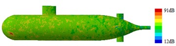
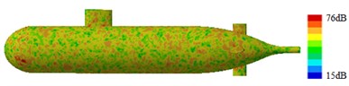
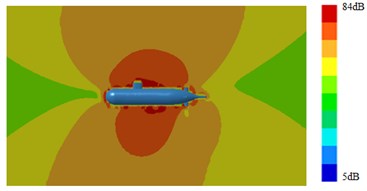
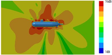
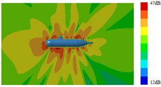
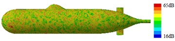
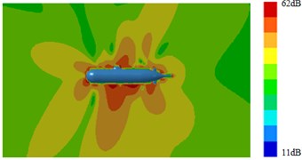
It was shown in Section 4.2 and Section 4.3 that pressure distribution and vorticity distribution on the surface of submarine with a Type 3 fairwater were obviously different from the other structures. And fluctuating pressure was the source of the radiation noise of submarines. Therefore, based on the above computational method of the sound field, surface sound pressure and radiation noise of the submarine with the improved fairwater were computed. Computation results were shown in Fig. 14, Fig. 15, Fig. 16 and Fig. 17. It was shown in comparison between Fig. 5, Fig. 14 and Fig. 16 that surface sound fields of submarines with three different structures of fairwaters were obviously different. However, with increase of the analyzed frequency, surface sound fields of three submarines tended to decrease. The sound pressure of Type 3 had minimum; Type 2 ranked the second place; the surface sound pressure of Type 1 had relatively maximum. It was shown in comparison between Fig. 6, Fig. 15 and Fig. 17 that the changing of fairwater had obvious influences on distribution and size of the whole radiation sound field of submarines.

Fig. 14Sound field on surface of type 2 submarine

a) 100 Hz

b) 1000 Hz

c) 2000 Hz

d) 5000 Hz

Fig. 15Radiation noises of type 2 submarine

a) 100 Hz

b) 1000 Hz

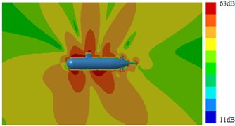
a) 100 Hz

b) 1000 Hz

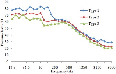
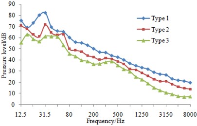
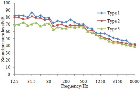
The radiation noise in 1/3 octave was also computed as shown in Fig. 18. It was indicated that both the fairwater with fillet and the streamline fairwater were reduced in terms of flow-induced noise. During the frequency band of 12.5 Hz~100 kHz, the fairwater with fillet was reduced by 2~5 dB and the streamline fairwater was reduced by 3~12 dB; and at the frequency band of 100 Hz~500 Hz, the fairwater with fillet was reduced by1~8 dB and the streamline fairwater was reduced by 2~10 dB. The total sound level of flow-induced noise was computed and obtained regarding three kinds of fairwaters at the frequency of 12.5 Hz~8000 Hz. In comparison with the original scheme, the total sound level of flow-induced noise was reduced by 5 dB in the fairwater with fillet, while that was reduced by 9 dB in the streamline fairwater. The computational method was verified in previous chapters, and the computational accuracy of three examples was basically same. Besides, the noise reduction effect was the comparison result of three fairwaters, which should be reliable.

Fig. 16Sound field on surface of type 3 submarine

a) 100 Hz

b) 1000 Hz

c) 2000 Hz

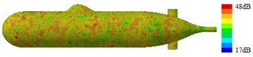
d) 5000 Hz

Fig. 17Radiation noises of type 3 submarine

a) 100 Hz

b) 1000 Hz

a) 100 Hz

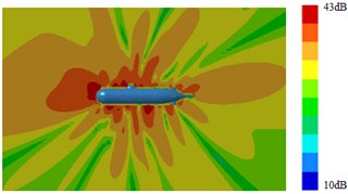
b) 1000 Hz

In conclusion, the fairwater with fillet or the streamline fairwater can significantly improve the flow quality, which enables the total sound level and spectral amplitude of both the pressure fluctuation and flow-induced noise to be dropped considerably.

Fig. 18Radiation noise of different fairwaters

5. Conclusions

At present, the research topic of this field is to conduct optimization design of submarines by using numerical simulation. Driven by the linear optimization and flow control of submarines, and to suppress vortex and reduce pressure fluctuations and flow-induced noise, fillets were installed on the front edge of a submarine fairwater and the streamline fairwater was designed in the paper. In addition, LES method was applied to conduct the numerical computation for the vortex flow field, wall pressure fluctuations as well as flow-induced noise of the original fairwater, the fairwater with fillet and the streamline fairwater. Furthermore, the impact and suppression effect of the fairwater shape on wall pressure fluctuations and flow-induced noise were analyzed. As shown from the results, the streamline fairwater can significantly improve the flow quality and the total sound pressure and spectral amplitude of the pressure fluctuations to be reduced considerably. The total sound level of pressure fluctuations was reduced by 2~21 dB in the streamline fairwater. And the total sound level of flow-induced noise was reduced by 9 dB. A technical support for the acoustic design and hydrodynamic design of new submarines can be provided by the paper.

References

Yu M. S., Wu Y. S., Pang Y. Z. A review of progress for hydrodynamic noise of ships. Journal of Ship Mechanics, Vol. 11, Issue 1, 2007, p. 152-158.

Search CrossRef
Wei Y., Wang Y. Unsteady hydrodynamics of blade forces and acoustic responses of a model scaled submarine excited by propeller's thrust and side-forces. Journal of Sound and Vibration, Vol. 332, Issue 8, 2013, p. 2038-2056.

Publisher
Arakeri V. H. Studies on scaling of flow noise received at the stagnation point of ax symmetric body. Journal of Sound and Vibration, Vol. 146, 1991, p. 449-462.

Publisher
Martin J. E., Michael T., Carrica P. M. Submarine maneuvers using direct overset simulation of appendages and propeller and coupled CFD/potential flow propeller solver. Journal of Ship Research, Vol. 59, Issue 1, 2015, p. 31-48.

Publisher
Hu Q. W. Research of Noise Mechanism of Submarine Sail Model. Harbin Engineering University, Harbin, 2007.

Search CrossRef
Skudrzyk E. J., Haddle G. P. Noise production in a turbulent boundary layer by smooth and rough surfaces. Journal of Sound and Vibration, Vol. 32, Issue 1, 1960, p. 19-34.

Publisher
Lu Y. T., Zhang H. X. Numerical simulation of flow-field and flow-noise of a fully appendage submarine. Journal of Vibration and Shock, Vol. 27, Issue 9, 2008, p. 142-146.

Search CrossRef
Zeng W. D., Wang Y. S. Numerical calculation of flow noise of submarine with full appendages. Acta Arm Amentar, Vol. 9, 2010, p. 1204-1208.

Search CrossRef
Crighton D. G. Goals for Computational Aero-Acoustics. Computational Acoustics: Algorithms and Applications, Elsevier-North Holland, Amsterdam, 1988, p. 3-20.

Search CrossRef
Colonius T., Lele S. K. Computational aero-acoustics: progress on nonlinear problems of sound generation. Progress in Aerospace Sciences, Vol. 40, Issue 6, 2004, p. 345-416.

Publisher
Zhang N., Shen H. C. Validation of numerical simulation on resistance and flow field of submarine and numerical optimization of submarine hull form. Journal of Ship Mechanics, Vol. 9, Issue 1, 2005, p. 1-13.

Search CrossRef

Cited by

The Generation Mechanism of the Flow-Induced Noise from a Sail Hull on the Scaled Submarine Model

Yongwei Liu | Yalin Li | Dejiang Shang

(2018)

About this article

Received

02 March 2016

Accepted

18 August 2016

Published

31 December 2016

SUBJECTS

Flow induced structural vibrations

DOI

https://doi.org/10.21595/jve.2016.16942

Keywords

fairwater

linear optimization

pressure fluctuations

flow-induced noise

This is an open access article distributed under the Creative Commons Attribution License, which permits unrestricted use, distribution, and reproduction in any medium, provided the original work is properly cited.

Previous article in issue Previous Next article in issue Next

Research article

2018 10 19

Parametric study of unsteady-flow-induced volute casing vibro-acoustics in a centrifugal fan

Jianhua Zhang, Wuli Chu, Yi Lv

Research article

2017 11 15

Numerical optimization for radiated noises of centrifugal pumps in the near-field and far-field based on a novel MLGA-PSO algorithm

Xue Yu Lu, Zheng Qiao Lu

Research article

2017 08 15

Influence of volute basic circle diameter on the pressure fluctuations and flow noise of a low specific speed sewage pump

Linwei Tan, Desheng Zhang, Weidong Shi, Ling Zhou, Xiaotong Cai

Research article

2016 08 15

Experimental and numerical investigation of interior flow-induced noise in pump as turbine

Liang Dong, Cui Dai, Hou-lin Liu, Fan-yu Kong

L. Huo and S.- Fei, “Design on the fairwater shape and its influence on the radiation noise of submarines,” Journal of Vibroengineering, Vol. 18, No. 8, pp. 5378–5389, Dec. 2016, https://doi.org/10.21595/jve.2016.16942

Copy Extrica

Copied to clipboard!

TY  - JOUR
DO  - 10.21595/jve.2016.16942
UR  - https://doi.org/10.21595/jve.2016.16942
TI  - Design on the fairwater shape and its influence on the radiation noise of submarines
T2  - Journal of Vibroengineering
AU  - Huo, Lin
AU  - Fei, Si-miao
PY  - 2016
DA  - 2016/12/31
PB  - JVE International Ltd.
SP  - 5378-5389
IS  - 8
VL  - 18
SN  - 1392-8716
ER  - 

Copy Ris

Copied to clipboard!

@article{Huo_2016,
	doi = {10.21595/jve.2016.16942},
	url = {https://doi.org/10.21595/jve.2016.16942},
	year = 2016,
	month = {dec},
	publisher = {{JVE} International Ltd.},
	volume = {18},
	number = {8},
	pages = {5378--5389},
	author = {Lin Huo and Si-miao Fei},
	title = {Design on the fairwater shape and its influence on the radiation noise of submarines},
	journal = {Journal of Vibroengineering}
}

Copy Bibtex

Copied to clipboard!

[1]L. Huo and S. Fei, “Design on the fairwater shape and its influence on the radiation noise of submarines,” Journal of Vibroengineering, vol. 18, no. 8, pp. 5378–5389, Dec. 2016, doi: 10.21595/jve.2016.16942.

Copy IEEE

Copied to clipboard!

Huo, Lin, and Si-miao Fei. “Design on the Fairwater Shape and Its Influence on the Radiation Noise of Submarines.” Journal of Vibroengineering 18, no. 8 (December 31, 2016): 5378–89. https://doi.org/10.21595/jve.2016.16942.

Copy Chicago

Copied to clipboard!

Design on the fairwater shape and its influence on the radiation noise of submarines

Abstract

1. Introduction

2. Numerical simulation method

2.1. Equation of large eddy simulation

2.2. Equation of acoustic analogy

2.3. Computational characteristic of flow-induced noise

2.4. Computational results of the flow field

3. Verification of numerical computation model

4. Suppression on submarine radiation noises

4.1. Flow fields of different fairwaters

4.2. Pressure fluctuations of different observation points for fairwaters

4.3. Radiation noises of different fairwaters

5. Conclusions

References

Cited by

About this article

Related Articles