Abstract
A general framework for investigating the on-load frequencies of roadway bridges under stochastic traffic flows was developed. The cellular automaton (CA) model was adopted to develop the stochastic traffic flow. The on-load natural frequencies of the bridge are analyzed statistically. The results show that the on-load frequencies of bridge are less than the corresponding natural frequencies of the bridge. For higher or lower traffic occupancies, the fluctuation of on-load natural frequencies of the bridge becomes smaller than that under the middle range of traffic flow densities. A linear relationship exists between the mean frequency difference and the traffic flow density, with the mean slope of regression lines for the first four natural frequencies being 0.0844. There is a stronger linear relationship between the mean frequency difference and the total traffic weight, with the mean slope being 0.482. Based on traffic flow density or total traffic weight on the bridge, it is possible to make an estimate of the effect of traffic flows on the on-load frequency of a reinforced concrete continuous beam bridge using the regression relationships.
1. Introduction
Studies of the dynamic behavior of bridges under moving vehicle loads have been undertaken for many years, especially for railway bridges [1-8] and numerous achievements have been achieved regarding the analysis of dynamic train-bridge interaction [1-5]. Some scholars have studied the on-load natural frequencies of railway bridges, focusing on the effect of trains on the natural frequencies of bridges, examining carriage masses coupled with a bridge through their suspension systems. Li et al. investigated the main factors that influence the resonant vibration and the relationship between the resonance speed and the natural frequencies of a girder bridge [8]. The results show that the fundamental natural frequency varies periodically as a train passes over the bridge. Ren et al. focused on continuous bridges, and some results show that the vertical train-bridge natural frequency periodically varies when trains are distributed on the whole bridge [7]. When the length of the train is shorter than that of the bridge, the periodic change of the vertical train-bridge natural frequency does not occur and then the vehicle-bridge system will not experience vertical resonance. Recently, the significance and the variation trends of the driving frequencies and dominant frequencies in a bridge response resulting from trainloads were examined by Lu et al. [6].
In recent years, there has been an increasing number of problems relating to highway bridges due to, in part, longe spans, high strength and light materials used in new bridges. Many researchers have recognized this problem, and most of their studies have focused on the dynamic analysis of highway bridges based on vehicle-bridge interaction [9-12]. Another important problem related to highway bridges is that bridges present decreasing natural frequencies when subjected to traffic flows. As a result, it is desirable that the frequency variation of bridges under traffic flows (namely on-load natural frequencies of roadway bridges) should be considered. Based on traffic-induced vibration tests on three bridges, the measured natural frequencies can change up to 5.4 % for short span bridges whose mass is relatively small [13]. The interaction between vehicular traffic and bridge vibration for a short span bridge was studied experimentally and analytically by Kwon et al. [14]. It was clear that the behavior of the bridge-vehicle system cannot be understood without taking the properties of the vehicle suspension for a heavily loaded vehicle into account. The relative and absolute frequency changes of damaged reinforced concrete bridge structures under moving vehicular loads are sensitive to the weight of the moving vehicle, and the frequency ratio between the vehicle and the bridge has some effect on them [15]. A theoretical framework has been presented for the variation in frequencies of vibration of the Vehicle-bridge interaction (VBI) system by Yang et al. [16-18], which indicates that the effect is crucial when the vehicle mass is not negligible compared to the bridge mass or when a resonance condition is approached.
Some researchers have examined the frequency variation of bridges under vehicle loads. For a train-bridge system [6-8], the train is modelled as multiple carriages (several masses or degrees-of-freedom systems) and the bridge modelled as a beam. For studying a vehicle-bridge system, similar to a train-bridge system, the vehicle has been modelled as a moving mass [18] or a several degrees-of-freedom system [15-17] and the bridge modelled as a beam. However, the vehicle-bridge system is different from the train-bridge system because: 1) many vehicles travelling on the roadway bridge are randomly distributed on bridges, while either one or two trains travelling on a railway bridge will be uniformly distributed, 2) the width of the roadway bridge is larger than that of a railway bridge, hence the mechanical characteristics of a roadway bridge are similar to those of a beam. Therefore, although the model of the vehicle-bridge system mentioned above can capture the physical essence of roadway bridge on-load natural frequencies, but it is almost impossible to be used to calculate the frequency variation of an actual roadway bridge under real traffic flows.
This paper presents a method for investigating the variation of natural frequencies of an actual roadway bridge under stochastic traffic loads. Section 2 presents a 3D finite model of a bridge developed in ANSYS [19]. Section 3 uses a cellular automaton (CA) model to develop the stochastic traffic flow on the roadway bridge [20]. This microscopic scale traffic flow simulation model has been widely used in the transportation field. Then, in Section 4, each vehicle in the stochastic traffic flow is modelled as a fixed mass, and the frequency of the roadway bridge at each time step, is calculated using ANSYS for the stochastic traffic flow across the bridge. This method makes it possible to calculate the on-load natural frequencies of the actual bridge under real traffic flows, which can potentially help bridge designers to consider the variation of bridge frequencies under traffic flows.
2. The FEM bridge model
In this study, the two-lane one-way Xiancun Bridge in Guangzhou, China, was investigated. It is a reinforced concrete, continuous box-girder bridge. The bridge has three spans, which are 55+85+55 m, with a total length of 195 m. The width of the bridge is 15 m, and its total weight is about 6.06×10⁶ kg. A schematic diagram of the bridge is shown in Fig. 1. ANSYS was used to construct a full 3-D FEM of the bridge.
Three different principal materials are used in the bridge for different structural elements: steel reinforced concrete, bituminous concrete, and rubber bearing are adopted as the box-girders, the pavement and the bridge supports. The mechanical properties of these materials are given in Table 1. The research focused on the natural frequency variation of the bridge; however, damping and nonlinear properties were not considered.
Solid elements were used to build the model, as shown in Fig. 2. There are a total of 26,296 elements and 50,459 nodes.
The first four modes and natural frequencies of the bridge were determined using the Block Lanczos method and are presented in Fig. 3 and in Table 2.
Fig. 1Schematic views of the bridge (unit: m)

a) Elevation
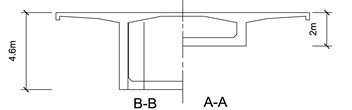
b) Typical cross sections
Fig. 2A FE model of the bridge (a half)
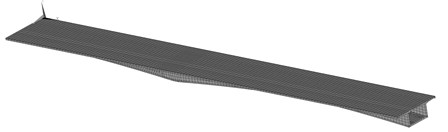
Fig. 3Mode shapes of the first four modes
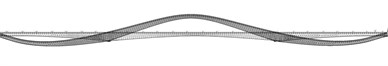
a) First mode shape
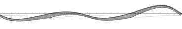
b) Second mode shape
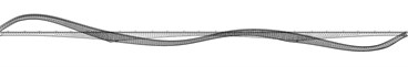
c) Third mode shape
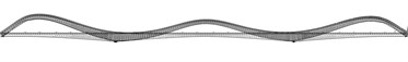
d) Fourth mode shape
Table 1Mechanical characteristics
Material | Steel reinforced Concrete | Bituminous concrete | Rubber bearing |
Young’s modulus (N/m2) | 3.7e10 | 4.5e9 | 3.7e8 |
Density (kg/m3) | 2500 | 2440 | 2150 |
Poisson ratio | 0.2 | 0.4 | 0.4 |
Table 2Natural frequencies of the first four modes
Mode No. | 1 | 2 | 3 | 4 |
Natural frequency (Hz) | 1.069 | 1.862 | 2.245 | 2.638 |
3. Stochastic traffic flow on the roadway
The cellular automaton (CA) model [20-22] was adopted to develop the stochastic traffic flow. The method is able to provide detailed instantaneous information about each vehicle through replicating major traffic phenomena on roadways. Thus it is an ideal technology to be integrated into advanced bridge analysis considering traffic flows in a more realistic manner. In the following sections, the theoretical basis of the proposed simulation framework for bridges with the CA model is briefly introduced, and the traffic flow on Xiancun bridge is simulated later.
3.1. Theoretical basis
The CA traffic model simulates stochastic traffic flows through time and space, with each lane being divided into cells of equal length. Each cell can be either empty or occupied by one vehicle at any time step. At each time step, a vehicle moves, accelerates, decelerates or changes lanes, based on some predefined rules [20-22]. The rules of a typical CA traffic model include: (1) rules of the single-lane CA model; and (2) the conditions for lane changing. Vehicle is taken as an example to introduce the CA traffic model rules. and are the velocities at time and respectively. and denote the locations of vehicleand the vehicle immediately ahead of vehicle . represents the maximum velocity. is the distance between vehicle and vehicle . denotes the randomization probability.
The rules for the single-lane CA model are shown as follows:
Rule 1: acceleration, if and .
Rule 2: deceleration , if .
Rule 3: randomization, .
Rule 4: vehicle motion. If the three conditions above are not satisfied, then .
Vehicle changes to the target lane with the probability of if all the following three criteria are satisfied:
Rule 5: .
Rule 6: , , denote the location of the nearest vehicle on the target lane moving ahead of vehicle .
Rule 7: , , is the location of the nearest vehicle on the target lane moving behind vehicle .
To complete the lane-changing simulation, the location and the velocity of vehicle will be updated through two sub-steps:
Step 1: vehicle moves to the target lane transversely without moving forward.
Step 2: vehicle moves forward obeying the single lane rule as illustrated above after moving into the target lane.
3.2. Traffic flow simulation on the bridge
In the study, the bridge is a two-lane one-way bridge. The total length of the bridge is 195 m (). Chen et al. (2011) suggested that approaching roadways on both sides of the bridge should be considered, because the actual traffic flow across a bridge is also affected by the traffic on the approaching roadways [22]. The approaching roadway has a length of 975 m () at each end of the bridge [22]. The length of ‘roadway-bridge-roadway’ system is therefore 2145 m. The bridge and the approaching roadways have the same number of available lanes. All the lanes on the bridge and the connecting roadways share the same width and each lane is divided into equally-spaced cells. The rules for the bridge and the approaching roadways are the same. The length of each cell () is set to be 7.5 m [22], which is the typical distance between the centers of two vehicles when the road is completely congested. Then, the number of cells in one lane is 286 (). The velocity limit is assumed to be 120 km/h, which is the typical speed limit on highways in China. The period of each time step is 1 s. So in the CA model can be computed accordingly:
In the following CA-based traffic flow simulation, a periodic boundary condition is adopted. The initial velocities of all the vehicles are randomly set among 0-4 (cell/s). The CA rules dictate the velocity of each individual vehicle according to the speed limit adaptively. The probability of braking () is 0.5. The probability of changing lane () is 0.8. Various vehicles on highways are grouped into eight categories, the weights of various vehicles being summarized in Table 3. The proportions of the vehicles from each category are assumed to be 0.125.
With the adoption of the periodic boundary condition, the traffic occupancy in the whole system remains constant for each simulation. Thirty-seven densities () have been considered, namely: 0.03, 0.05, 0.07, 0.09, 0.11, 0.13, 0.15, 0.17, 0.20, 0.22, 0.24, 0.26, 0.28, 0.30, 0.32, 0.34, 0.36, 0.38, 0.40, 0.42, 0.44, 0.46, 0.48, 0.50, 0.52, 0.54, 0.56, 0.58, 0.60, 0.65, 0.70, 0.75, 0.80, 0.85, 0.90, 0.95 and 1.00. Three densities 0.15, 0.24 and 0.36 correspond to service levels B, D and F. Other densities have been proposed for this research. 1.00 indicates that every cell of Xiancun bridge is occupied by a vehicle. The observation of the traffic flow starts after 10 ( is the number of cells in one lane, here 286) when the traffic flow is believed to have become steady [22]. The traffic flow starting from 3000 s will be presented in the following sections.
Table 3The weight of various vehicles
Categories | Car | Mini bus | Light bus | Bus | Mini truck | Light truck | Truck | Heavy truck |
Weight (kg) | 2000 | 7220 | 10000 | 20000 | 10000 | 15000 | 25000 | 32000 |
The typical two-lane traffic simulation of a ‘roadway-bridge-roadway’ system is conducted and the results are shown in Fig. 4, where the time versus space information of the simulated traffic flow on one lane is given. The -axis shows the physical location of each vehicle on the ‘roadway-bridge-roadway’. The -axis shows that the time range after 3000 s of simulation has elapsed. At any time instant on the -axis, the information of the physical distribution of each vehicle along the spatial simulation region (-axis) can be found by drawing a line horizontally. Similarly, at any spatial location on the -axis, the time-variant information of vehicles at one particular location can be retrieved by drawing a line vertically.
Fig. 4 shows four different situations at four different densities. The operational condition of the bridge for free flow is at 0.0. As the density increases, traffic congestion occurs. The ability to maneuver is severely restricted due to traffic congestion at 0.15. At 0.24 and 0.36, the traffic flow breaks-down, and vehicles arrive at a rate greater than the rate at which they are discharged. Operations within queues are highly unstable, vehicles experiencing brief periods of movement followed by stoppages.
Fig. 4Traffic flow simulation result
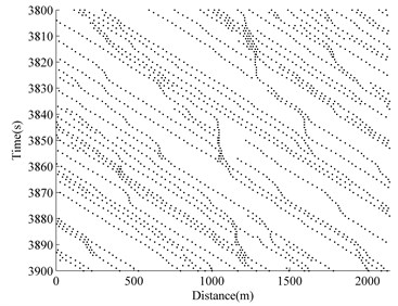
a) 0.07
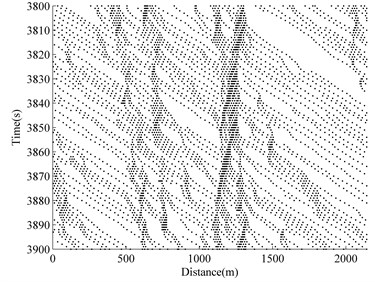
b) 0.15
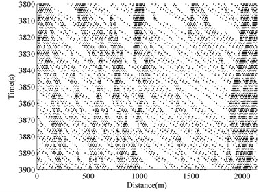
c) 0.24
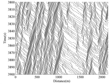
d) 0.36
4. Time-variant natural frequencies of the bridge
Actually, the frequency variation of Xiancun bridge under traffic loads is not obvious, because Xiancun bridge is a reinforced concrete girder bridge and the vehicle mass is lighter compared to the bridge mass. However, it is sufficient to examine the method suggested in the paper to analyze the natural frequencies of the roadway bridge under stochastic traffic flows.
When the vehicle on the bridge is modelled as a mass, then, the force acting on the bridge is equal to:
where is the transversal dynamic deflection of the bridge structure, is the mass of the vehicle, is the acceleration of gravity, is the Dirac delta function, and are the velocity and the acceleration of the vehicle, respectively.
In general, the effect of the second (Coriolis forces), third (centripetal forces) and fourth term (the acceleration component forces) in the bracket on the right-hand side of Eq. (1) on the vehicle-bridge interaction can be neglected [23, 24], then, Eq. (2) is simplified as:
From the simplified force acting on the beam in Eq. (3), it can be concluded that the on-load natural frequencies of the bridge at time is equal to the frequencies of beam with a fixed mass at . Therefore, in the following studies on the on-load natural frequencies of the bridge, the Coriolis, centripetal and acceleration force components are not considered, i.e., each vehicle in the stochastic traffic flow is modelled as a fixed mass at each time step and the coupling between the bridge and vehicles is not considered.
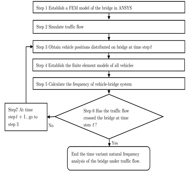
For the general framework of investigating the on-load frequencies of roadway bridges under stochastic traffic flows, the CA model was adopted to simulate traffic flows across the bridge, and FEM method was used to simulate the bridge. Then, the simulated traffic flow acted as loads to pass through the bridge, the frequency of the traffic flow-bridge system at each time step is calculated. The following is the detailed procedure for determining time variant natural frequencies of the bridge under traffic flows.
Step 1: Establishing the FE model of the bridge in ANSYS.
Step 2: Simulating traffic flows across the bridge based on CA traffic flow simulation technology.
Step 3: Obtaining positions of all vehicles distributed on the bridge at time step from traffic flow simulation results.
Step 4: Establishing the FE models of all vehicles on the FEM model of the bridge according to the position of vehicles and vehicle types. MASS 21 is adopted to simulate the vehicle.
Step 5: Calculating the frequency of the traffic flow-bridge system at time step . Note that each vehicle in the stochastic traffic flow is modelled as a fixed mass.
Step 6: Checking the traffic flow. If the traffic flow crosses the bridge, the time variant natural frequencies of the bridge under traffic flows finish.
Step 7: At time step , returning to step 3 and repeating the procedure until the traffic flow crosses the bridge.
Fig. 5 is a flowchart illustrating this procedure.
Due to the stochastic nature of the traffic flow across the bridge, the on-load natural frequencies of the bridge, at any one moment, are usually different. Fig. 6 gives the natural frequencies versus time for the 0.00, 0.03, 0.15, 0.36 and 0.60 conditions. Figs. 6(a)-6(d) show the first four natural frequencies. Legend 0.00 represents no vehicles on the bridge. The on-load frequencies of the bridge are less than the corresponding order natural frequencies for 0.00. From Fig. 6, as the traffic density increases, the natural frequencies decrease in general. The natural frequencies under the 0.03 condition are equal to the natural frequencies of the empty bridge at some time intervals, such as [14 s, 25 s], which indicates that there are no vehicles on the bridge at those times. Due to many trucks and heavy trucks for 0.36 at around 70 seconds, the natural frequencies are greater than for 0.60, which illustrates one effect of the total traffic weight on the natural frequencies of bridges. However, the exact time period is different for different natural frequencies presented in Fig. 6, which indicates the influence of vehicle distribution.
To investigate the effect of stochastic traffic on different modes of the bridge, the time-history results for the absolute differences between the natural frequencies of the bridge and the bridge with vehicles for 0.15 are shown in Fig. 7. The mean values of the curves of absolute difference vs. time step for the first four natural frequencies are 0.012, 0.022, 0.025 and 0.032 Hz. The effect of vehicles on the higher modes of the bridge is more significant than on the lower modes, from the point of view of absolute difference. Based on the simulation of the stochastic traffic flow, the cumulative traffic weight from all the vehicles on the bridge can be calculated at any instant. The time-history results for 0.15 are shown in Fig. 8. It can be seen that the total traffic weight on the bridge generally has some variation over time due to the stochastic nature of the traffic flow. By carefully comparing this with Fig. 7, it can be seen that the absolute difference vs. time step follows the same trend as total traffic weight vs. time step.
Fig. 5Procedure to determine time variant natural frequencies of bridge under traffic flow
Due to the probabilistic nature of the traffic flow on the bridge, it can be found that the frequencies of the bridge with vehicles have some variations over time for a given traffic density. For different traffic densities, the on-load natural frequencies of the bridge are statistically analyzed. The mean natural frequency vs. traffic flow density curves for the first four natural frequencies are plotted in Fig. 9. It can be seen that the on-load natural frequencies of the bridge have some variations with traffic flow density. Similar to the results shown in Fig. 6, it is found from Fig. 9 that the mean natural frequencies decrease when the traffic flow densities increase.
Fig. 6Variations of the first four frequencies with time as the vehicles pass over the bridge
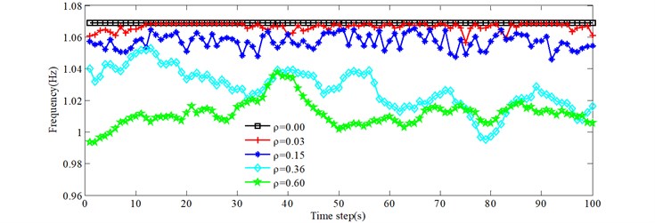
a) 1st natural frequency
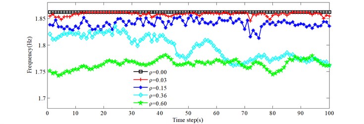
b) 2nd natural frequency
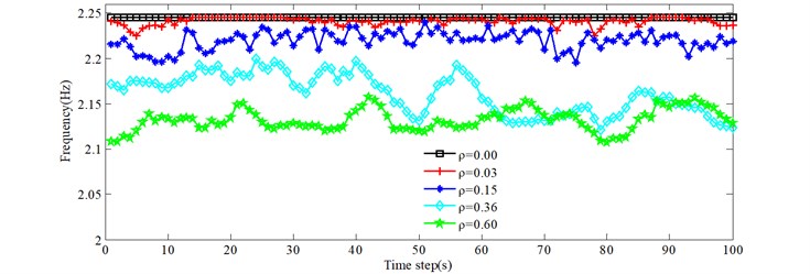
c) 3rd natural frequency
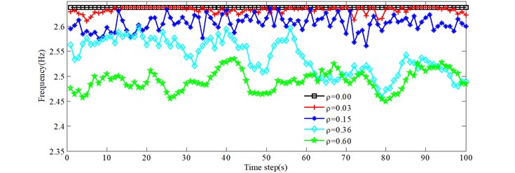
d) 4th natural frequency
Fig. 10 shows the standard deviation of on-load natural frequency versus traffic flow density for the first four natural frequencies. Fluctuations of standard deviation for the on-load frequencies of the bridge with various traffic densities can be observed in Fig. 10. It is found that the fluctuations of on-load frequencies of the bridge are smaller for both high and low traffic flow densities than in the middle range. To a certain extent, the higher standard deviations of on-load frequencies of the bridge may indicate more variations of the dynamic impacts on the bridge induced by traffic.
Fig. 7Effect of stochastic traffic on different modes of the bridge (ρ= 0.15)
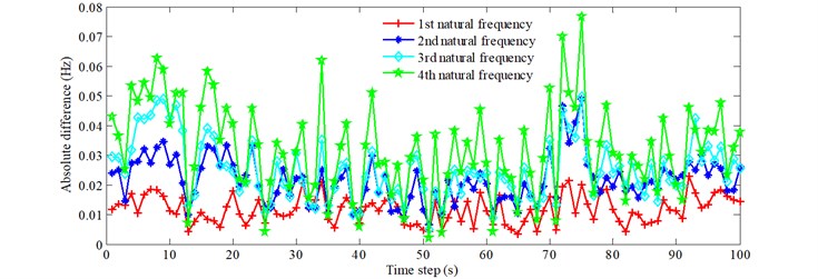
Fig. 8Effect of total traffic weight on different modes of the bridge (ρ= 0.15)
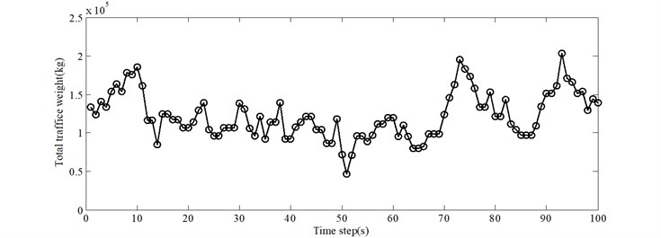
Fig. 9Mean natural frequency vs. traffic flow density
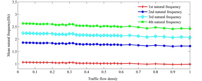
Fig. 11 gives the results of the mean value of the total traffic weight () under different traffic flow densities. In general, the total traffic weight increases as the traffic density increases. However, various vehicles with different weights in the traffic flow may mean that the total traffic weight is not always increasing monotonically as the traffic flow density increases, as shown in Fig. 11.
The relationship between the dimensionless mean frequency difference () and the traffic flow density () is studied for various natural frequencies (Fig. 12). for a traffic flow density is defined as follows:
in which represents th natural frequency of the bridge, is the mean value of th on-load natural frequency of the bridge under a traffic flow density.
Fig. 10Standard deviation of on-load natural frequency vs. traffic flow density
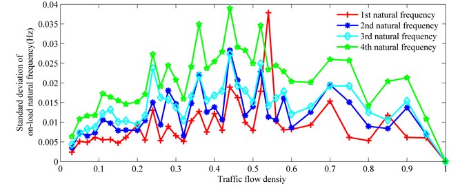
Fig. 11Mean total traffic weight vs. traffic flow density
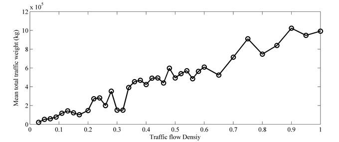
Fig. 12Mean frequency difference vs. traffic flow density
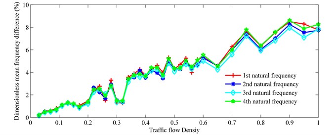
As displayed in Fig. 12, the difference between for various natural frequencies is minor. Fig. 12 shows that increases as increases, and a linear relationship exists between them. The linear correlation coefficients between and for various natural frequencies are presented in Table 4. Curve fitting, using least-squares linear regression, was carried out. The slopes of the lines for various natural frequencies are presented in Table 5. The slope differences between different natural frequencies are minor. The mean slope of all fitted lines is 0.0844. Due to the similar mechanical characteristics for different reinforced concrete continuous beam bridges, the mean slope can be used to roughly estimate the on-load frequency of this type of bridge according to the traffic flow density.
Table 4Linear correlation coefficient
Mode No. | 1 | 2 | 3 | 4 |
Linear correlation coefficient | 0.962 | 0.970 | 0.970 | 0.972 |
Table 5The slope of the fitted line
Mode No. | 1 | 2 | 3 | 4 |
Slope | 0.0867 | 0.0830 | 0.0807 | 0.0875 |
From the comparison of Figs. 11 and 12, a strong linear relationship exists between and , despite the stochastic distribution of vehicles on the bridges. This is verified by Fig. 13 which shows the relationship between the dimensionless mean frequency difference () and the dimensionless traffic total weight difference (). Data are rearranged according to the ascending order of total traffic weight in Fig. 13. The dimensionless traffic total weight difference () is defined as follows:
in which represents the total weight of the bridge (6.06×10⁶ kg), is the mean value of total traffic flow weight for a given traffic flow density.
The correlation coefficients between and , for various natural frequencies, are presented in Table 6. Compared to Table 4, a stronger linear relationship between and is displayed. Curve fitting using least-squares linear regression was again undertaken. The slopes of the fitted lines for various natural frequencies are presented in Table 7. The slope differences between different natural frequencies are minor. The mean slope of all the fitted lines is 0.482. Actually, the mean slope may also be used to estimate (approximately) the on-load frequency of a reinforced concrete continuous beam bridge according to the total traffic weight on the bridge.
Fig. 13Frequency difference vs. traffic flow density
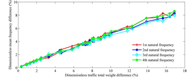
Table 6Linear correlation coefficient
Mode No. | 1 | 2 | 3 | 4 |
Linear correlation coefficient | 0.996 | 0.997 | 0.997 | 0.998 |
Table 7Slopes of the fitted line based on linear regression
Mode No. | 1 | 2 | 3 | 4 |
Slope | 0.508 | 0.483 | 0.470 | 0.508 |
5. Conclusions
Based on traffic flow simulation technology, a general framework for investigating the variations of natural frequencies of a roadway bridge under stochastic traffic loading has been developed. Due to the probabilistic nature of the traffic flow on the bridge, the on-load natural frequencies of the bridge induced by stochastic traffic flow vary over time. Following the development of the methodology, the on-load natural frequencies of the bridge are statistically analyzed. The major findings are summarized as follows:
1) The on-load frequencies of the bridge under stochastic traffic flow are less than the corresponding natural frequencies of the empty bridge. In general, the natural frequencies decrease as the values of the traffic density increase. Total traffic weight and vehicle distribution influence the on-load natural frequencies of the bridge.
2) From the point of view of absolute differences, the effects of vehicles on the higher modes of the bridge are more significant than the effects on the lower modes. The total traffic weight on the bridge has some variation over time, due to the stochastic nature of the traffic flow.
3) The mean natural frequencies decrease when the traffic flow densities increase. The fluctuations of the on-load frequencies of the bridge are smaller for both high and low traffic flow densities than for the middle range of traffic flow densities. To a certain extent, the higher standard deviations of the on-load frequencies of the bridge may mean greater variations of the dynamic impacts on the bridge induced by traffic.
4) In general, the total traffic weight increases as the traffic densities increase. However, various vehicles, with different weights in the traffic flow, may mean that total traffic weight does not always increase monotonically as the traffic flow density increases.
5) A linear relationship exists between the mean frequency difference and the traffic flow density. Based on least-squares linear curve fitting, the mean slope of all fitted lines is 0.0844, which means that the on-load frequencies of the roadway bridge can be approximately determined when the traffic flow density on this bridge is known.
6) A strong linear relationship exists between mean frequency difference and total traffic weight, despite the stochastic distribution of vehicles on the bridge. Based on least-squares linear curve fitting, the mean slope of all fitted lines is 0.482, which means that the on-load frequencies of the roadway bridge can be approximately determined when the total traffic weight on this bridge is known.
According to the method in the paper, it is only necessary to ascertain the distribution of vehicles on the bridge at each instant when calculating the bridge on-load natural frequencies, which makes it possible to calculate the actual bridge on-load natural frequencies under real traffic flow. This will greatly simplify the calculation of bridge on-load natural frequencies under actual traffic flow, which will be helpful for bridge designers considering the variation of bridge frequencies under stochastic traffic flow. However, the model is not validated by the field measurement until now, which will be performed in the next step.
References
-
Dimitrakopoulos E. G., Zeng Q. Three-dimensional dynamic analysis scheme for the interaction between trains and curved railway bridges. Computers and Structures, Vol. 149, 2015, p. 43-60.
-
Mellat P., Andersson A., Pettersson L., Karoumi R. Dynamic behavior of a short span soil-steel composite bridge for high-speed railways. Field measurements and FE-analysis. Engineering Structures, Vol. 69, Issue 15, 2014, p. 49-61.
-
Liu K., Zhou H., Shi G., Wang Y. Q., Shi Y. J., Roeck G. D. Fatigue assessment of a composite railway bridge for high speed trains. Part II: Conditions for which a dynamic analysis is needed. Journal of Constructional Steel Research, Vol. 82, 2013, p. 246-254.
-
Zambrano A. Determination of the critical loading conditions for bridges under crossing trains. Engineering Structures, Vol. 33, Issue 2, 2011, p. 320-329.
-
Zhang N., Xia H., Roeck G. D. Dynamic analysis of a train-bridge system under multi-support seismic excitations. Journal of Mechanical Science and Technology, Vol. 24, Issue 11, 2010, p. 2181-2188.
-
Lu Y., Mao L., Woodward P. Frequency characteristics of railway bridge response to moving trains with consideration of train mass. Engineering Structures, Vol. 42, 2012, p. 9-22.
-
Ren J. Y., Su M. B., Zeng Q. Y. Vertical load-carrying natural frequency of railway continuous steel truss bridges. 7th International Conference on Traffic and Transportation Studies, 2010, p. 1387-1398.
-
Li J. Z., Su M. B., Fan L. C. Natural Frequency of railway girder bridges under vehicle loads. Journal of Bridge Engineering, Vol. 8, Issue 4, 2003, p. 199-203.
-
Gao Q. F., Wang Z. L., Liu C. G., Li J., Jia H. Y., Zhong J. F. Dynamic responses of a three-span continuous girder bridge with variable cross-section based on vehicle-bridge coupled vibration analysis. The IES Journal Part A: Civil and Structural Engineering, Vol. 8, Issue 2, 2015, p. 1-10.
-
Ettefagh M. M., Behkamkia D., Pedrammehr S., Asadi K. Reliability analysis of the bridge dynamic response in a stochastic vehicle-bridge interaction. KSCE Journal of Civil Engineering, Vol. 19, Issue 1, 2015, p. 220-232.
-
Gui S. R., Liu L., Chen S. S., Zhao H. Research on models of a highway bridge subjected to a moving vehicle based on the LS-DYNA simulator. Journal of Highway and Transportation Research and Development, Vol. 8, Issue 3, 2014, p. 76-82.
-
Gao Q. F., Wang Z. L., Guo B. Q., Chen C. Dynamic responses of simply supported girder bridges to moving vehicular loads based on mathematical methods. Mathematical Problems in Engineering, 2014, p. 1-22.
-
Kim C. Y., Jung D. S., Kim Kwon N. S. S. D., Feng M. Q. Effect of vehicle weight on natural frequencies of bridges measured from traffic-induced vibration. Earthquake Engineering and Engineering Vibration, Vol. 2, Issue 1, 2003, p. 109-115.
-
Kwon S.-D., Kim C. Y., Chang S. P. Change of modal parameters of bridge due to vehicle pass. IMAC-23: Conference and Exposition on Structural Dynamic, Orlando, 2005, p. 213-219.
-
Law S. S., Zhu X. Q. Dynamic behaviour of damaged concrete bridge structures under moving vehicular loads. Engineering Structures, Vol. 26, Issue 9, 2004, p. 1279-1293.
-
Yang Y. B., Cheng M. C., Chang K. C. Frequency variation in vehicle bridge interaction systems. International Journal of Structural Stability and Dynamics, Vol. 13, Issue 2, 2013, p. 1-22.
-
Tan G. J., Cheng Y. C., Zhao H., Liu F. S. Research on the influence law of vehicles to the natural frequency of highway simply supported girder bridges. ICCTP – Integrated Transportation Systems – Green, Intelligent, Reliable ASCE, Beijing, 2010, p. 3201-3208.
-
Zarfam R., Khaloo A. R., Nikkhoo A. On the response spectrum of Euler-Bernoulli beams with a moving mass and horizontal support excitation. Mechanics Research Communications, Vol. 47, 2013, p. 77-83.
-
ANSYS Modeling and Meshing Guide. ANSYS Release 11.0[M/CD], ANSYS Inc., 2008.
-
Nagel K., Schreckenberg M. A cellular automaton model for freeway traffic. Journal of Phys I France, Vol. 2, Issue 12, 1992, p. 2221-2229.
-
Li X. G., Jia B., Gao Z. Y., Jiang R. A realistic two-lane cellular automata traffic model considering aggressive lane-changing behaviour of fast vehicle. Physica A, Vol. 367, 2006, p. 479-486.
-
Chen S. R., Wu J. Modelling stochastic live load for long-span bridge based on microscopic traffic flow simulation. Computers and Structures, Vol. 89, Issue 9, 2011, p. 813-824.
-
Mahmoud M. A., Zaid M. A. A. Dynamic response of a beam with a crack subject to a moving mass. Journal of Sound and Vibration, Vol. 256, Issue 4, 2002, p. 591-603.
-
Michaltsos G., Sophianopoulos D., Kounadis A. N. The effect of a moving mass and other parameters on the dynamic response of a simply supported beam. Journal of Sound and Vibration, Vol. 191, Issue 3, 1996, p. 357-362.
About this article

This work is supported by the China National Natural Fund (Project No. 51222801, 51178126, 51208125), the Science and Technology Program of Guangzhou (Project No. 2013J2200074), Science and Technology Planning Project of Guangdong Province (2016B050501004) and China Scholarship Council. This financial support is gratefully acknowledged.
Mao Ye developed the concept and designed the study. Xiangxiang Chen carried out the analysis of the time-variant natural frequencies of the bridge and wrote the manuscript. Min Ren assisted with the analysis of the stochastic traffic. Baoxing Cao assisted with the FEM bridge model. Shifan Huang assisted with the analysis of the stochastic traffic.
