Numerical simulation of dynamic response characteristics for launch and recovery system under random irregular wave

Jin, Yongping; Wan, Buyan; Liu, Deshun; Peng, Youduo; Cai, Zhihua; Dong, Jianghui

doi:10.21595/jve.2016.16955

Journal of Vibroengineering

Browse Journal

Submit article

Published: 31 December 2016

Check for updates

Numerical simulation of dynamic response characteristics for launch and recovery system under random irregular wave

Yongping Jin¹

Buyan Wan²

Deshun Liu³

Youduo Peng⁴

Zhihua Cai⁵

Jianghui Dong⁶

¹College of Mechanical and Electrical Engineering, Central South University, Changsha, 410083, China

^{2, 3, 4}Hunan Province Engineering Laboratory of Marine Mineral Resources Exploration Equipment and Technology, Hunan University of Science and Technology, Xiangtan, 411201, China

⁵College of Electromechanical Engineering, Hunan University of Science and Technology, Xiangtan, 411201, China

⁶School of Natural and Built Environments, University of South Australia, Adelaide, SA 5095, Australia

Corresponding Author:

Jianghui Dong

Cite the article Download PDF

Downloads 1655

WoS Core Citations 4

CrossRef Citations 4

Abstract

Based on the rain-flow counting method, a new random numerical simulation method for evaluating dynamic response characteristics of a launch and recovery system is presented in this study. It takes a random irregular wave as an input, and the random distribution characteristics of the dynamic responses of the launch and recovery system of a seafloor drill is analyzed by using the rain-flow counting method. The nonlinear coupling mechanisms among the movements of the ship, the umbilical cable, and the seafloor drill caused by random irregular wave are investigated. A dynamic model that considers the influence of the seawater resistance on the launch and recovery system of seafloor drill is established. Then, significant wave heights are used to produce excitation of the random irregular wave, and the corresponding dynamic random responses of the launch and recovery system are calculated and analyzed. At the same time, the movement of the seafloor drill and the tension of the umbilical cable are calculated and analyzed for the cases of seafloor drill at different water depths. This method provides a new tool for evaluating the dynamic response characteristics of launch and recovery system of other seafloor equipment under random irregular wave.

1. Introduction

Hoisting machinery is widely used to transfer cargo and other equipment from and to various locations in industrial field, such as land hoisting machinery and marine hoisting machinery. Compared to land hoisting machinery, marine hoisting machinery is more complicated due to the influence of many factors, like wave, wind, and ocean currents, which typically impose a greater impact on safety and efficiency of the hoisting operations. Recently, a number of studies involving the dynamic response characteristics among the movement of the ship, the cable, and the cargo of the marine hoisting machinery have been reported in the literature [1-6]. However, in most of these studies, the cargo is not in touch with the seawater and its lifting height is normally from ten to several hundred meters in the process of the hoisting. In order to conduct marine geologic survey, marine environment exploration and other marine scientific investigation, some deep-sea equipment, such as seafloor drill, deep-sea mining vehicle and remote operated vehicle (ROV), requires to be operated near seafloor with different water depths (sometimes, the water depth is more than thousands of meters). Due to the combined effects of wave, wind, and ocean currents, the ship motions are complicated. As a result, when the deep-sea equipment reaches the seafloor, its actual touchdown location may be quite different than the expected one. In addition, the movement of deep-sea equipment will lead to a significant vibration of the cable and make the cable fracture and failure [7-9].

In most studies, regular wave is typically chosen as an external excitation to analyze the dynamic responses of the marine hoisting machinery system. However, this is not true for the actual hoisting operation environment. Actually, real ocean waves are random and irregular, and these wave patterns are constituted by a series of random wavelengths and random wave amplitudes. Based on the statistical analysis of a large amount of random irregular wave patterns, all of them actually have some statistical regularities. For different random irregular wave patterns, the significant wave height could be considered as a statistical characteristic value. Furthermore, in most previous research, the random irregular wave followed the normal distribution, and the significant wave height of the random irregular wave followed the Rayleigh distribution.

In this paper, based on the rain-flow counting method, a new random numerical simulation method is applied to assess dynamic response characteristics of the launch and recovery system. A random wave is used as an input, and the random distribution of dynamic responses of the launch and recovery system are calculated and analyzed. Analysis results can provide theoretical guidance for the estimation of heave compensation and the constant-tension control of the umbilical cable. In addition, random irregular wave was typically chosen as an external excitation to analyze the dynamic responses of the launch and recovery system in this study. We just presented the dynamic response characteristics of the launch and recovery system and the statistic distributed regularity of the responses of the movement of the ship, the umbilical cable, and the seafloor drill in the sea state 4 condition. It is a practical trial to apply statistics analysis to evaluate the dynamic responses of the marine hoisting machinery under random irregular wave.

2. Dynamical model of launch and recovery system

2.1. Model description

Fig. 1 shows a sketch of a launch and recovery system with a seafloor drill. This system mainly includes a ship, a marine winch, an umbilical cable, a hoist boom, and a seafloor drill. Two assumptions are applied for the following analysis in this study:

(1) The elastic deformation of the umbilical cable and the rotation of the seafloor drill are ignored.

(2) The hoist boom is assumed as a rigid rod.

Fig. 1Sketch of launch and recovery system of seafloor drill

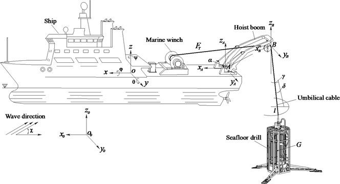
In Fig. 1 three coordinate systems are introduced to describe the launch and recovery system of the seafloor drill. The inertial coordinate system, $O_{0}$ - $x_{0} y_{0} z_{0}$ , is fixed to the ground. The coordinate system of the ship, $O$ - $x y z$ , is fixed to and moves with the ship. Point $A$ is located at the center of the rotation axis of the hoist boom, and point $B$ is located at the hoisting point of the hoist boom. The distance from point $A$ to the origin of the coordinate system of the ship is defined as $L_{O A}$ , and the distance from point $B$ to point $A$ is defined as $L_{A B}$ . $α$ is the angle anticlockwise from $A B$ to the axis $x$ .

In order to describe the orientation of the umbilical cable in $O_{0}$ - $x_{0} y_{0} z_{0}$ , two angles, represented by $γ$ and $δ$ are used (Fig. 1). These two angles will be referred to as the in-plane pendulum angle and the out-of-plane pendulum angle, respectively.

2.2. Ship motions and external loads

The differential equations of heaving, rolling, and pitching motions of the ship caused by irregular waves can be described as follows [10]:

1

\{\begin{array}{l} (m_{s h i p} + Δ m_{z z}) \ddot{z} + A_{1 z} \dot{z} + A_{2 z} z + A_{3 z} \ddot{θ} + A_{4 z} \dot{θ} + A_{5 z} θ = F_{z}, \\ (J_{φ φ} + Δ J_{φ φ}) \ddot{φ} + B_{1 φ} |\dot{φ}| \dot{φ} + B_{2 φ} φ + B_{3 φ} φ^{3} = M_{φ}, \\ (J_{θ θ} + Δ J_{θ θ}) \ddot{θ} + C_{1 θ} \dot{θ} + C_{2 θ} θ + C_{3 θ} \ddot{z} + C_{4 θ} \dot{z} + C_{5 θ} z = M_{θ}, \end{array}

where $m_{s h i p}$ is the mass of the ship, $∆ m_{z z}$ is the added mass due to heaving motion, $A_{1 z}$ , $A_{2 z}$ , $A_{3 z}$ , $A_{4 z}$ and $A_{5 z}$ are hydrodynamic coefficients of the heaving motion. $J_{φ φ}$ and $∆ J_{φ φ}$ are inertia moment and the additional inertia moment due to the rolling motion, respectively. $B_{1 φ}$ is the damping moment coefficient of the rolling motion, $B_{2 φ}$ and $B_{3 φ}$ are restore moment coefficients of the rolling motion. $J_{θ θ}$ and $∆ J_{θ θ}$ are inertia moment and the additional inertia moment due to the pitching motion. $C_{1 θ}$ , $C_{2 θ}$ , $C_{3 θ}$ , $C_{4 θ}$ and $C_{5 θ}$ are hydrodynamic coefficients of the pitching motion. $F_{z}$ , $M_{φ}$ and $M_{θ}$ are the interference forces of the heaving motion, interference moments of the rolling and the pitching motion, respectively. Some coefficients in Eq. (1) could be calculated based on empirical equations [11, 12].

In $O$ - $x y z$ , the hydrodynamic pressure at position ( $x$ , $y$ , $z$ ) can be expressed as:

2

Δ p (x, y, z) = - ρ g e^{- k z} ξ (t),

where $ρ$ is the density of seawater, $g$ is the gravity constant, $k$ is the wave number, $ξ (t)$ is the wave surface coordinate.

Based on the Froude-Krylov assumption, the interference force of heaving motion, interference moments of rolling motion and pitching motion can be described as follows:

3

\{\begin{array}{l} F_{z} = ∭_{V} \frac{\partial Δ p}{\partial z} d V, \\ M_{φ} = ∭_{V} (\frac{\partial Δ p}{\partial y} z - \frac{\partial Δ p}{\partial z} y) d V, \\ M_{θ} = ∭_{V} (\frac{\partial Δ p}{\partial z} x - \frac{\partial Δ p}{\partial x} z) d V . \end{array}

Substituting Eq. (2) into Eq. (3), and the ship was simplified as a box structure, one has:

4

\begin{array}{l} \{\begin{array}{l} F_{z} = - \frac{ρ g}{a b} \sum_{i = 1}^{n} \frac{s i n (L a ω_{i}^{2}) s i n (B b ω_{i}^{2})}{ω_{i}^{4}} ζ_{i} (1 - e x p (- \frac{ω_{i}^{2} T}{g})) \cdot c o s (ω_{i} (1 - 2 v a ω_{i}) t - ε_{i}), \\ M_{φ} = (\begin{matrix} \frac{ρ g}{a} \sum_{i = 1}^{n} \frac{ζ_{i} s i n (L a ω_{i}^{2}) s i n (ω_{i} (1 - 2 v a ω_{i}) t - ε_{i})}{ω_{i}^{4}} (1 - e x p (- \frac{ω_{i}^{2} T}{g})) \\ \cdot (\frac{s i n (B b ω_{i}^{2})}{2 b^{2} ω_{i}^{2}} - \frac{B c o s (B b ω_{i}^{2})}{2 b} - 2 g z_{b} s i n (B b ω_{i}^{2})) \end{matrix}), \\ M_{θ} = (\begin{matrix} \frac{ρ g}{2 a b} \sum_{i = 1}^{n} \frac{ζ_{i}}{ω_{i}^{4}} (1 - e x p (- \frac{ω_{i}^{2} T}{g})) (\frac{s i n (L a ω_{i}^{2})}{a ω_{i}^{2}} - L c o s (L a ω_{i}^{2})) \\ ∙ s i n (B b ω_{i}^{2}) s i n (ω_{i} (1 - 2 v a ω_{i}) t - ε_{i}) \end{matrix}), \end{array} \\ a = \frac{c o s χ}{2 g}, b = \frac{s i n χ}{2 g}, \end{array}

where $B$ , $T$ , and $L$ are breadth, draught, and length of the ship, respectively. $v$ is the forward speed in the $x$ direction of the ship, $z_{b}$ is the vertical coordinate of the ship’s buoyancy center.

2.3. Dynamic equation of launch and recovery system

The homogeneous transformation matrix from $O$ - $x y z$ to $O_{0}$ - $x_{0} y_{0} z_{0}$ is:

5

T = T (x, y, z) R (x, φ) R (y, θ)

= [\begin{array}{l} 1 & 0 & 0 & x \\ 0 & 1 & 0 & y \\ 0 & 0 & 1 & z \\ 0 & 0 & 0 & 1 \end{array}] [\begin{array}{l} 1 & 0 & 0 & 0 \\ 0 & c o s φ & - s i n φ & 0 \\ 0 & s i n φ & c o s φ & 0 \\ 0 & 0 & 0 & 1 \end{array}] [\begin{matrix} c o s θ & 0 & s i n θ & 0 \\ 0 & 1 & 0 & 0 \\ - s i n θ & 0 & c o s θ & 0 \\ 0 & 0 & 0 & 1 \end{matrix}]

= [\begin{matrix} c o s θ & s i n θ s i n φ & s i n θ c o s φ & x \\ 0 & c o s φ & - s i n φ & y \\ - s i n θ & c o s θ s i n φ & c o s θ c o s φ & z \\ 0 & 0 & 0 & 1 \end{matrix}] .

Consequently, the hoisting point of the hoist boom $B (x_{B}, y_{B}, z_{B})$ in $O_{0}$ - $x_{0} y_{0} z_{0}$ can be described as following:

6

[\begin{array}{l} x_{B} \\ y_{B} \\ z_{B} \\ 1 \end{array}] = [\begin{matrix} c o s θ & s i n θ s i n φ & s i n θ c o s φ & x \\ 0 & c o s φ & - s i n φ & y \\ - s i n θ & c o s θ s i n φ & c o s θ c o s φ & z \\ 0 & 0 & 0 & 1 \end{matrix}] [\begin{matrix} - L_{O A} - L_{A B} s i n α \\ 0 \\ L_{A B} c o s α \\ 1 \end{matrix}]

= [\begin{matrix} x - L_{O A} c o s θ + L_{A B} c o s α c o s θ + L_{A B} s i n α s i n θ c o s φ \\ y - L_{A B} s i n α s i n φ \\ z + L_{O A} s i n θ - L_{A B} c o s α s i n θ + L_{A B} s i n α c o s θ c o s φ \\ 1 \end{matrix}] .

The center of gravity of the seafloor drill $G (x_{G}, y_{G}, z_{G})$ is derived as following:

7

[\begin{matrix} x_{G} \\ y_{G} \\ z_{G} \\ 1 \end{matrix}] = [\begin{matrix} x_{B} \\ y_{B} \\ z_{B} \\ 1 \end{matrix}] + [\begin{matrix} - l s i n γ c o s δ \\ l s i n δ \\ - l c o s γ c o s δ \\ 1 \end{matrix}]

= [\begin{matrix} x - L_{O A} c o s θ + L_{A B} c o s α c o s θ + L_{A B} s i n α s i n θ c o s φ - l s i n γ c o s δ \\ y - L_{A B} s i n α s i n φ + l s i n δ \\ z + L_{O A} s i n θ - L_{A B} c o s α s i n θ + L_{A B} s i n α c o s θ c o s φ - l c o s γ c o s δ \\ 1 \end{matrix}],

where $z$ , $φ$ , $θ$ , $γ$ and $δ$ are the parameters depended on time, $l$ is the length of the umbilical cable, $α$ is assumed to be constant. By differentiating the position of the center of gravity of the seafloor drill $G (x_{G}, y_{G}, z_{G})$ , the velocity is derived from Eq. (7):

8

[\begin{array}{l} {\dot{x}}_{G} \\ {\dot{y}}_{G} \\ {\dot{z}}_{G} \end{array}] = [\begin{matrix} \begin{matrix} \dot{x} + L_{O A} \dot{θ} s i n θ - L_{A B} \dot{θ} c o s α s i n θ + L_{A B} \dot{θ} s i n α c o s θ c o s φ - L_{A B} \dot{φ} s i n α s i n θ s i n φ \\ - \dot{l} s i n γ c o s δ - l \dot{γ} c o s γ c o s δ + l \dot{δ} s i n γ s i n δ \end{matrix} \\ \dot{y} - L_{A B} \dot{φ} s i n α c o s φ + \dot{l} s i n δ + l \dot{δ} c o s δ \\ \begin{matrix} \dot{z} + L_{O A} \dot{θ} c o s θ - L_{A B} \dot{θ} c o s α c o s θ - L_{A B} \dot{θ} s i n α s i n θ c o s φ - L_{A B} \dot{φ} s i n α c o s θ s i n φ \\ - \dot{l} c o s γ c o s δ + l \dot{γ} s i n γ c o s δ + l \dot{δ} c o s γ s i n δ \end{matrix} \end{matrix}] .

The kinetic energy of the launch and recovery system can be obtained as follows:

9

T = \frac{1}{2} m_{d r i l l} ({\dot{x}}_{G}^{2} + {\dot{y}}_{G}^{2} + {\dot{z}}_{G}^{2}) = \frac{1}{2} m_{d r i l l} [{\dot{x}}^{2} + {\dot{z}}^{2} + {\dot{l}}^{2} + l^{2} {\dot{δ}}^{2} + l^{2} {\dot{γ}}^{2} c o s^{2} δ

+ {\dot{θ}}^{2} (L_{O A}^{2} + L_{A B}^{2} c o s^{2} α + L_{A B}^{2} s i n^{2} α c o s^{2} φ - 2 L_{A O} L_{A B} c o s α)

+ 2 \dot{x} (L_{O A} \dot{θ} s i n θ - L_{A B} \dot{θ} c o s α s i n θ + L_{A B} \dot{θ} s i n α c o s θ c o s φ - L_{A B} \dot{φ} s i n α s i n θ s i n φ + c_{1})

+ 2 \dot{y} (\dot{l} s i n δ + l \dot{δ} c o s δ - L_{A B} \dot{φ} s i n α c o s φ)

+ 2 \dot{z} (L_{O A} \dot{θ} c o s θ - L_{A B} \dot{θ} c o s α c o s θ - L_{A B} \dot{θ} s i n α s i n θ c o s φ - L_{A B} \dot{φ} s i n α c o s θ s i n φ + c_{2})

+ 2 c_{1} (L_{O A} \dot{θ} s i n θ - L_{A B} \dot{θ} c o s α s i n θ + L_{A B} \dot{θ} s i n α c o s θ c o s φ - L_{A B} \dot{φ} s i n α s i n θ s i n φ)

+ 2 c_{2} (L_{O A} \dot{θ} c o s θ - L_{A B} \dot{θ} c o s α c o s θ - L_{A B} \dot{θ} s i n α s i n θ c o s φ - L_{A B} \dot{φ} s i n α c o s θ s i n φ)

- 2 L_{O A} L_{A B} \dot{θ} \dot{φ} s i n α s i n φ + 2 L_{A B}^{2} \dot{θ} \dot{φ} s i n α c o s α s i n φ

- 2 L_{A B} \dot{φ} s i n α c o s φ (\dot{l} s i n δ + l \dot{δ} c o s δ) + 2 l \dot{l} \dot{δ} s i n δ c o s δ],

c_{1} = - \dot{l} s i n γ c o s δ - l \dot{γ} c o s γ c o s δ + l \dot{δ} s i n γ s i n δ,

c_{2} = - \dot{l} c o s γ c o s δ + l \dot{γ} s i n γ c o s δ + l \dot{δ} c o s γ s i n δ,

where $m_{d r i l l}$ is the mass of the seafloor drill.

The potential energy of the launch and recovery system is obtained:

10

U = m_{d r i l l} g (z + L_{O A} s i n θ - L_{A B} c o s α s i n θ - L_{A B} s i n α c o s θ c o s φ - l c o s γ c o s δ) .

The Lagrangian function of the launch and recovery system can be expressed as:

11

L = T - U .

The Lagrange equation is:

12

\frac{d}{d t} (\frac{\partial L}{\partial {\dot{q}}_{k}}) - \frac{\partial L}{\partial q_{k}} = Q_{k},

where $q_{k}$ , ${\dot{q}}_{k}$ and $Q_{k}$ are general coordinates, general velocities and general forces of the launch and recovery system, respectively.

Substituting Eq. (11) into Eq. (12), one has:

13

m_{d r i l l} [\ddot{z} + L_{O A} \ddot{θ} c o s θ - L_{O A} {\dot{θ}}^{2} s i n θ - L_{A B} \ddot{θ} c o s α c o s θ + L_{A B} {\dot{θ}}^{2} c o s α s i n θ

- L_{A B} \ddot{θ} s i n α s i n θ c o s φ - L_{A B} \ddot{φ} s i n α c o s θ s i n φ + 2 L_{A B} \dot{θ} \dot{φ} s i n α s i n θ s i n φ

+ L_{A B} ({\dot{φ}}^{2} - {\dot{θ}}^{2}) s i n α c o s θ c o s φ - \ddot{l} c o s γ c o s δ + 2 \dot{l} \dot{γ} s i n γ c o s δ + 2 \dot{l} \dot{δ} c o s γ s i n δ

+ l \ddot{γ} s i n γ c o s δ + l \ddot{δ} c o s γ s i n δ + l c o s γ c o s δ ({\dot{γ}}^{2} + {\dot{δ}}^{2}) - 2 l \dot{γ} \dot{δ} s i n γ s i n δ - g] = f_{z},

14

m_{d r i l l} [l^{2} \ddot{γ} c o s^{2} δ + 2 l \dot{l} \dot{γ} c o s^{2} δ - 2 l^{2} \dot{γ} \dot{δ} s i n δ c o s δ - l c o s γ c o s δ (\ddot{x} + L_{O A} \ddot{θ} s i n θ

+ L_{O A} {\dot{θ}}^{2} c o s θ - L_{A B} \ddot{θ} c o s α s i n θ - L_{A B} {\dot{θ}}^{2} c o s α c o s θ + L_{A B} \ddot{θ} s i n α c o s θ c o s φ

- L_{A B} \ddot{φ} s i n α s i n θ s i n φ - 2 L_{A B} \dot{θ} \dot{φ} s i n α c o s θ s i n φ - L_{A B} ({\dot{θ}}^{2} + {\dot{φ}}^{2}) s i n α s i n θ c o s φ)

+ l s i n γ c o s δ (\ddot{z} + g + L_{O A} \ddot{θ} c o s θ - L_{O A} {\dot{θ}}^{2} s i n θ - L_{A B} \ddot{θ} c o s α c o s θ + L_{A B} {\dot{θ}}^{2} c o s α s i n θ

- L_{A B} \ddot{θ} s i n α s i n θ c o s φ - L_{A B} \ddot{φ} s i n α c o s θ s i n φ

+ 2 L_{A B} \dot{θ} \dot{φ} s i n α s i n θ s i n φ + L_{A B} ({\dot{φ}}^{2} - {\dot{θ}}^{2}) s i n α c o s θ c o s φ)] = f_{γ},

15

m_{d r i l l} [\ddot{δ} l^{2} + 2 l \dot{δ} \dot{l} + l^{2} {\dot{γ}}^{2} s i n δ c o s δ + l s i n γ s i n δ (\ddot{x} + L_{O A} \ddot{θ} s i n θ + L_{O A} {\dot{θ}}^{2} c o s θ

- L_{A B} \ddot{θ} c o s α s i n θ - L_{A B} {\dot{θ}}^{2} c o s α c o s θ + L_{A B} \ddot{θ} s i n α c o s θ c o s φ - L_{A B} \ddot{φ} s i n α s i n θ s i n φ

- 2 L_{A B} \dot{θ} \dot{φ} s i n α c o s θ s i n φ - L_{A B} ({\dot{θ}}^{2} + {\dot{φ}}^{2}) s i n α s i n θ c o s φ)

+ l c o s γ s i n δ (\ddot{z} + g + L_{O A} \ddot{θ} c o s θ - L_{O A} {\dot{θ}}^{2} s i n θ - L_{A B} \ddot{θ} c o s α c o s θ

+ L_{A B} {\dot{θ}}^{2} c o s α s i n θ - L_{A B} \ddot{θ} s i n α s i n θ c o s φ - L_{A B} \ddot{φ} s i n α c o s θ s i n φ

+ 2 L_{A B} \dot{θ} \dot{φ} s i n α s i n θ s i n φ + L_{A B} ({\dot{φ}}^{2} - {\dot{θ}}^{2}) s i n α c o s θ c o s φ)

+ \ddot{y} l c o s δ - L_{A B} l \ddot{φ} s i n α c o s φ c o s δ + L_{A B} l {\dot{φ}}^{2} s i n α s i n φ c o s δ + {\dot{l}}^{2} s i n δ c o s δ] = f_{δ} .

The generalized force of the launch and recovery system is mainly the seawater resistance, it can be expressed as:

16

[\begin{array}{l} f_{z} \\ f_{γ} \\ f_{δ} \end{array}] = - \frac{ρ}{2} [\begin{matrix} C_{z} S_{z} |{\dot{z}}_{G}| {\dot{z}}_{G} \\ C_{x} S_{x} |{\dot{x}}_{G}| {\dot{x}}_{G} \\ C_{y} S_{y} |{\dot{y}}_{G}| {\dot{y}}_{G} \end{matrix}],

where $ρ$ is the density of seawater. $C_{x}$ , $C_{y}$ and $C_{z}$ are resistance coefficients of the movement of the seafloor drill in three directions, and $S_{x}$ , $S_{y}$ and $S_{z}$ are resistance surface areas of seafloor drill in three directions, respectively.

2.4. The tension of umbilical cable

According to Newton’s second law, the movement of the seafloor drill can be expressed as:

17

m_{d r i l l} \cdot [\begin{array}{l} {\ddot{x}}_{G} \\ {\ddot{y}}_{G} \\ {\ddot{z}}_{G} \end{array}] = [\begin{matrix} F_{T} s i n γ c o s δ - \frac{1}{2} ρ C_{x} S_{x} |{\dot{x}}_{G}| {\dot{x}}_{G} - F_{T} s i n δ + \frac{1}{2} ρ C_{y} S_{y} |{\dot{y}}_{G}| {\dot{y}}_{G} \\ F_{T} c o s γ c o s δ + ρ g V_{d r i l l} - m_{d r i l l} g - \frac{1}{2} ρ C_{z} S_{z} |{\dot{z}}_{G}| {\dot{z}}_{G} \end{matrix}],

where $F_{T}$ is the tension of the umbilical cable, $V_{d r i l l}$ is the volume of the seafloor drill.

Based on Eq. (17), the tension of the umbilical cable $F_{T}$ can be expressed as:

18

F_{T} = (m_{d r i l l} \cdot {\ddot{x}}_{G} + \frac{1}{2} ρ C_{x} S_{x} |{\dot{x}}_{G}| {\dot{x}}_{G}) s i n γ c o s δ - (m_{d r i l l} \cdot {\ddot{y}}_{G} - \frac{1}{2} ρ C_{y} S_{y} |{\dot{y}}_{G}| {\dot{y}}_{G}) s i n δ

+ (m_{d r i l l} \cdot {\ddot{z}}_{G} + \frac{1}{2} ρ C_{z} S_{z} |{\dot{z}}_{G}| {\dot{z}}_{G}) c o s γ c o s δ + (m_{d r i l l} g - ρ g V_{d r i l l}) c o s γ c o s δ .

3. Dynamic random numerical simulation method

3.1. Random irregular wave model

The random irregular wave is assumed as a superposition of a series of linear waves [13-15]. The wave coordinate $ξ (t)$ of the random irregular wave can be expressed as:

19

ξ (t) = \sum_{j = 1}^{N} ζ_{j} c o s (k_{j} x c o s χ - k_{j} y s i n χ - ω_{j} t + ε_{j}),

where $ζ_{j}$ , $ω_{j}$ and $k_{j}$ are the wave amplitude, frequency and wave number for wave component $j$ , respectively. $ε_{j}$ is the random phase angle of the wave component $j$ with uniform distribution between 0 and 2 $π$ , $χ$ is the wave angle from the wave direction to the negative direction of the axis $x$ .

Wave spectrum $S (ω_{j})$ is statistic information of random irregular wave and the relationship between wave amplitude $ζ_{j}$ and $S (ω_{j})$ can be written as:

20

ζ_{j} = \sqrt{2 S (ω_{j}) Δ ω_{j}} = \sqrt{2 S (ω_{j}) (ω_{j} - ω_{j - 1})} .

Then Eq. (19) can be expressed as:

21

ξ (t) = \sum_{j = 1}^{N} \sqrt{2 S (ω_{j}) Δ ω_{j}} c o s (k_{j} x c o s χ - k_{j} y s i n χ - ω_{j} t + ε_{j}) .

Here, a Pierson-Moscowitz (P-M) wave spectrum is selected to describe the wave spectrum [16]. The P-M wave spectrum is defined as:

22

S (ω_{j}) = \frac{0.78}{ω_{j}^{5}} e x p (\frac{- 3.11}{ω_{j}^{4} H_{1 / 3}^{2}}),

where $H_{1 / 3}$ is the significant wave height.

Theoretically, the frequency range of P-M wave spectrum is from zero to infinity, but random irregular wave is a stationary stochastic process that belongs to narrow-band spectrum, and its energy mainly concentrated on a narrow frequency band. Therefore, during the numerical simulation process of random irregular wave, the maximum and minimum frequencies $ω_{m a x}$ and $ω_{m i n}$ are chosen, and the frequency range from $ω_{m i n}$ to $ω_{m a x}$ is discretized through adopting uniformly space sampling. This method not only can guarantee enough accuracy of numerical simulation, but also can significantly improve the efficiency of numerical simulation.

3.2. Significant wave height of random irregular wave

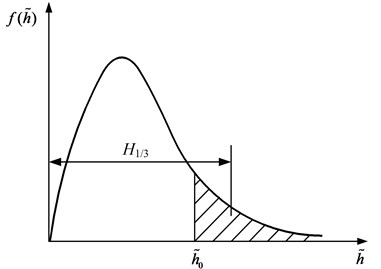
Different sea-states could be represented by different significant wave heights. For example, the significant wave height of sea-state 4 is 2.1 m. In physical oceanography, the significant wave height (illustrated in Fig. 2) is defined, traditionally, as the mean wave height of the highest third of the waves. In Fig. 2, $H_{1 / 3}$ is defined as the significant wave height.

For the continuous density function of the wave height, the significant wave height can be expressed as:

23

H_{1 / 3} = 3 \int_{{\tilde{h}}_{0}}^{+ \infty} \tilde{h} f (\tilde{h}) d \tilde{h},

where $f (\tilde{h})$ is the density function of wave height, ${\tilde{h}}_{0}$ is the dividing point, and ${\tilde{h}}_{0}$ satisfy the following expression:

24

\int_{{\tilde{h}}_{0}}^{+ \infty} f (\tilde{h}) d \tilde{h} = \frac{1}{3} .

Fig. 2The definition of significant wave height

Firstly, based on computer-based simulation, an expected value of significant wave height ( $H_{1 / 3}$ ) for a given sea-state is applied to generate a series of random irregular wave. Then, after classifying and analyzing the wave height, the mean wave height of the highest third of the random irregular wave $({\bar{\tilde{h}}}_{i_{1 / 3}})$ for component $i$ could be calculated. Theoretically, when the simulation time $t$ approaches infinity, the ${\bar{\tilde{h}}}_{i_{1 / 3}}$ will approach the given value of significant wave height ( $H_{1 / 3}$ ). However, typically it will consume quite long simulation time. Therefore, in this paper, we define a terminal condition to stop the numerical simulation:

Given a steady-state deviation $∆$ , when the deviation between the mean wave height of the highest third of the random irregular wave and the given value of significant wave height ( $H_{1 / 3}$ ) is less than the given steady-state deviation $∆$ for 10 times continuously, the numerical simulation will stop, and the corresponding wave coordinate is taken as the wave coordinate of the significant wave height of the given sea-state. The terminal condition can be expressed as:

25

|{\bar{\tilde{h}}}_{i_{1 / 3}} - H_{1 / 3}| < Δ, |{\bar{\tilde{h}}}_{i + 1_{1 / 3}} - H_{1 / 3}| < Δ, \dots, |{\bar{\tilde{h}}}_{i + 9_{1 / 3}} - H_{1 / 3}| < Δ .

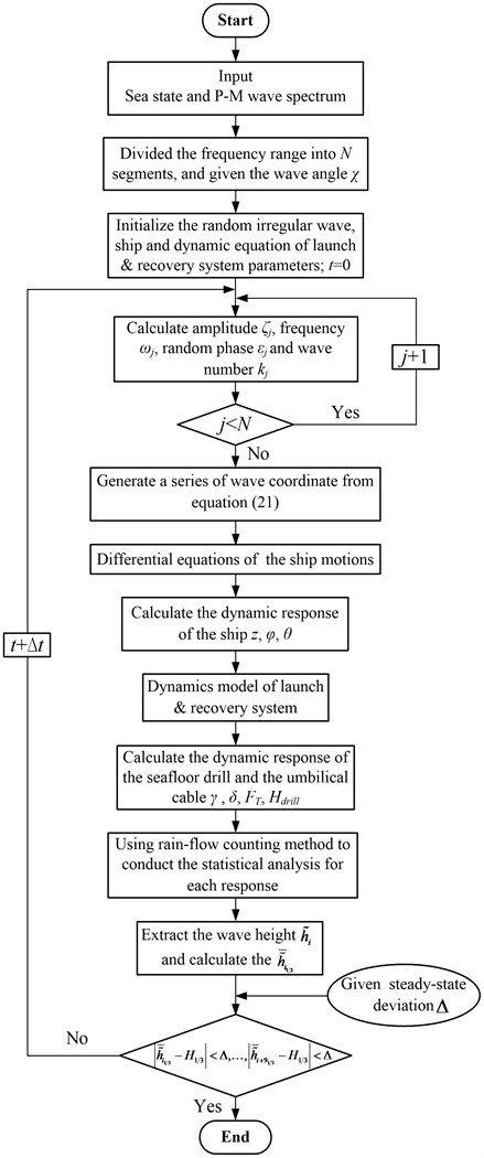
3.3. Dynamic random numerical simulation program

Step 1. Input an expected value of significant wave height ( $H_{1 / 3}$ ) for a given sea-state, and the corresponding P-M wave spectrum.

Step 2. Divide the frequency range ( $ω_{m i n}$ - $ω_{m a x}$ ) into $N$ segments, and specify the wave angle $χ$ .

Step 3. Initialize the random irregular wave, the dynamic equation of launch and recovery system parameters and the simulation time $t =$ 0.

Step 4. Calculate wave amplitude $ζ_{j}$ , wave frequency $ω_{j}$ , random phase $ε_{j}$ andwave number $k_{j}$ .

Step 5. Apply $ζ_{j}$ , $ω_{j}$ , $ε_{j}$ , $k_{j}$ and $χ$ to the wave coordinate Eq. (21) to generate wave coordinate.

Step 6. Calculate the dynamic responses of the ship (heaving motion $z$ , rolling motion $φ$ and pitching motion $θ$ ) from ship motion equations.

Step 7. Calculate the dynamic responses of the seafloor drill and the umbilical cable (in-plane angle $γ$ , out-of-plane angle $δ$ , tension of the umbilical cable $F_{T}$ , and heaving motion of the seafloor drill $H_{d r i l l}$ ) from Eqs. (13) to (18).

Step 8. Use rain-flow counting method [17-19] to analyze wave coordinate $ξ (t)$ of the random irregular wave, the dynamic responses of the ship, the seafloor drill and the umbilical cable; calculate their statistical distribution and characteristic values.

Step 9. Extract the wave heights of the random irregular wave ${\tilde{h}}_{1}$ , ${\tilde{h}}_{2}$ , ${\tilde{h}}_{3}$ , …, ${\tilde{h}}_{i}$ in descending order; then, calculate the mean wave height ${\bar{\tilde{h}}}_{i_{1 / 3}}$ of the highest third of them.

Step 10. Specify a steady-state deviation $∆$ as a terminal condition for the numerical simulation, when the following conditions are reached, the numerical simulation will stop, and the corresponding wave coordinate is taken as the wave coordinate of the significant wave height of the given sea-state:

|{\bar{\tilde{h}}}_{i_{1 / 3}} - H_{1 / 3}| < Δ, |{\bar{\tilde{h}}}_{i + 1_{1 / 3}} - H_{1 / 3}| < Δ, \dots, |{\bar{\tilde{h}}}_{i + 9_{1 / 3}} - H_{1 / 3}| < Δ .

Step 11. If the terminal condition is not satisfied, then $t = t + ∆ t$ ( $∆ t$ is the time step of numerical simulation) will come back to Step 4 to continue generate the random irregular wave until satisfy the simulation terminal condition.

Fig. 3 shows the flow chart of the dynamic random numerical simulation of the launch and recovery system.

4. Random numerical simulation of the launch and recovery system

Based on the procedure discussed in the previous section, a calculation case of a scientific research ship under sea-state 4 is demonstrated in this section. The simulation parameters of launch and recovery system are given in Table 1.

Table 1Simulation parameters

Parameters	Values
Ship length (m)	73.3
Ship breadth (m)	10.2
Ship draught (m)	3.4
Ship mass (kg)	1200000
$L_{O A}$ (m)	35.5
$L_{A B}$ (m)	6
Angle $a$ (°)	135
Vertical coordinate $z_{b}$ (m)	0.62
Seafloor drill mass (kg)	8000
Seafloor drill volume (m³)	1.56
Resistance coefficient $C_{x}$	1.67
Resistance coefficient $C_{y}$	1.67
Resistance coefficient $C_{z}$	1.67
Resistance surface areas $S_{x}$	8.35
Resistance surface areas $S_{y}$	8.5
Resistance surface areas $S_{z}$	4.67
Density of water $ρ$ (kg/m³)	1000

In the process of launch and recovery of the seafloor drill, the ship has been anchored, so we let the forward speed $v =$ 0.

Fig. 3Flow chart of the dynamic random numerical simulation of the launch and recovery system

4.1. Random irregular wave generation

The significant wave height of sea-state 4 is specified to 2.1 m. The steady-state deviation $∆$ is 0.001 m. The frequency range from $ω_{m i n}$ to $ω_{m a x}$ is (0.3-3) rad/s. The wave direction $χ$ is 30°, and $N$ is 30. The time step of simulation is set to be $∆ t =$ 0.2 seconds. The convergence of the wave heights of the random irregular wave to 2.1 m is shown in Fig. 4. The total simulation time to achieve this is 35008 seconds.

Fig. 4The convergence of the wave heights of the random irregular wave to 2.1 m

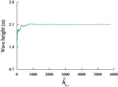
Fig. 5(a) shows a part of the wave coordinate of a random irregular wave. Based on the rain-flow counting method, it can be seen that the wave coordinate of the random irregular wave follows the normal distribution with mean $μ =$ 0.0078 and standard deviation $σ =$ 0.847. The probability density function of the wave coordinate is shown in Fig. 5(a).

Fig. 5The dynamic response of the wave coordinate

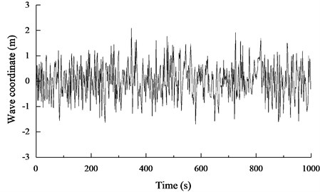
a) A part of the wave coordinate of the random irregular wave

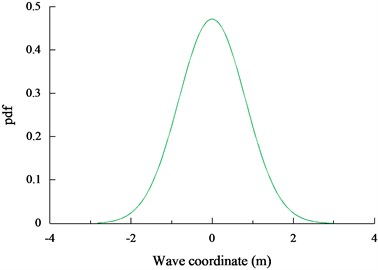
b) The probability density function of the wave coordinate

4.2. The dynamic response of the ship

Fig. 6(a) shows a part of the dynamic response of the ship heaving motion. Based on the rain-flow counting method, it can be seen that the ship appeared an irregular heaving motion under this random irregular wave. The ship heaving motion follows the normal distribution with $μ =$ 0.00001 and $σ =$ 0.3479. The probability density function of the ship heaving motion is shown in Fig. 6(b).

Fig. 6The dynamic response of the ship heaving motion

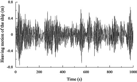
a) A part of the response curve of the ship heaving motion

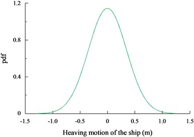
b) The probability density function of the ship heaving motion

Similarly, the dynamic response data of the ship rolling motion and the ship pitching motion can be obtained by using the rain-flow counting method. The ship rolling motion also follows the normal distribution with $μ =$ 0.0003 and $σ =$ 1.1245. The ship pitching motion follows the normal distribution with $μ =$ 0.00009 and $σ =$ 0.0248.

Compared the dynamic response data of the ship rolling motion with that of the ship pitching motion, it can be found that the standard deviation of the ship rolling motion is larger than the standard deviation of the ship pitching motion, and this is due to the length of the ship is larger than the width of the ship, which makes the pitching motion is more stable than the rolling motion.

4.3. The dynamic response of the seafloor drill and the umbilical cable

Figs. 7(a)-(d) show a part of the dynamic responses of the in-plane, out-of-plane pendulum angle ( $γ$ and $δ$ ), the tension of the umbilical cable ( $F_{T}$ ), and the heaving motion of the seafloor drill ( $H_{d r i l l}$ ) for the seafloor drill at the depth of 10 m, respectively. Based on the rain-flow counting method, it can be seen that the distribution of the angle $γ$ , the angle $δ$ , the $F_{T}$ and the $H_{d r i l l}$ for the seafloor drill at the depth of 10 m follow normal distributions with $μ =$ –0.0149° and $σ =$ 1.7117; $μ =$ 0.1792° and $σ =$ 8.3203; $μ =$ 67237.9 N, and $σ =$ 30115.8; $μ =$ 0.0980 m, and $σ =$ 0.3674, respectively.

Figs. 8(a)-(d) show the probability density functions of the angle $γ$ , the angle $δ$ , the $F_{T}$ and the $H_{d r i l l}$ for the seafloor drill at the depth of 10 m, respectively.

4.4. The dynamic response of the seafloor drill and the umbilical cable under different water depths

The mean values and the standard deviations of the angle $γ$ , the angle $δ$ , the $F_{T}$ and the $H_{d r i l l}$ for the seafloor drill at the depth of 10 m, 100 m and 1000 m are listed in Table 2.

Fig. 7A part of the dynamic response of the seafloor drill and the umbilical cable for the seafloor drill at the depth of 10 meters

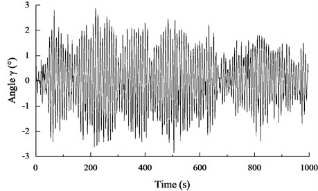
a) A part of the response curve of the pendulum angle $γ$

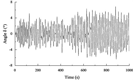
b) A part of the response curve of the pendulum angle $δ$

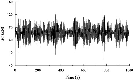
c) A part of the response curve of the tension of the umbilical cable

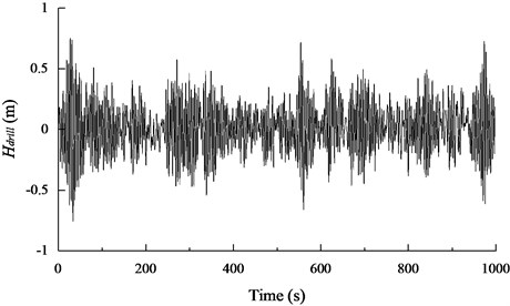
d) A part of the response curve of the heaving motion of the seafloor drill

Fig. 8The probability density function of the of the seafloor drill and the umbilical cable for the seafloor drill at the depth of 10 meter

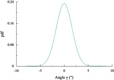
a) The probability density function of the pendulum angle $γ$

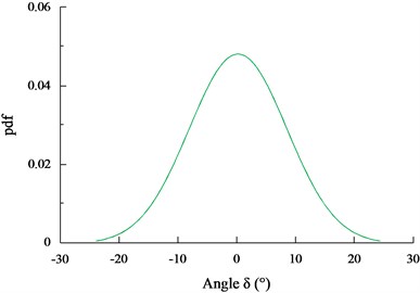
b) The probability density function of the pendulum angle $δ$

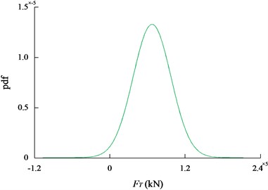
c) The probability density function of the tension of the umbilical cable

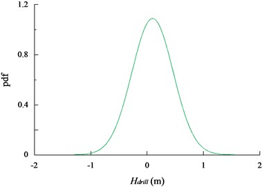
d) The probability density function of the heaving motion of the seafloor drill

Table 2The dynamic response of the seafloor drill and the umbilical cable under different water depths

	Water depth 10 m		Water depth 100 m		Water depth 1000 m
	Mean	Standard deviation	Mean	Standard deviation	Mean	Standard deviation
Angle $γ$ (°)	–0.0149	1.7117	0.0097	0.1636	0.0005	0.0783
Angle $δ$ (°)	0.1792	8.3203	–0.0807	3.1106	–0.0079	0.2113
$F_{T}$ (kN)	67237.9	30115.8	67266.1	30462.4	66865.2	31099.6
$H_{d r i l l}$ (m)	0.0980	0.3674	0.0886	0.3616	0.0055	0.3482

By comparing the mean values and the standard deviations of the angle $γ$ , the angle $δ$ , the $F_{T}$ and the $H_{d r i l l}$ at the different depths, it could be concluded that the increase of the water depth will decrease the amplitude of the angle $γ$ , the angle $δ$ . the change of water depth does not significantly affect the variation of $F_{T}$ and $H_{d r i l l}$ . Compared with the standard deviation of the heaving motion of the ship, the standard deviation of the heaving motion of the seafloor drill is more than times larger than it for the seafloor drill at water depth 10 meters, 100 meters and 1000 meters. This is due to the hoist boom was fixed in the quarter-deck of the ship, which make the pitching motion of the ship has the most significant influence on the heaving motion of the seafloor drill.

5. Conclusions

In the current study, a dynamic model that considers the influence of the seawater resistance on the launch and recovery system of a seafloor drill is established. By applying a random irregular wave as an external excitation, the random distribution characteristics of the dynamic responses of the launch and recovery system are analyzed and calculated by using the rain-flow counting method. This study shows that the ship appeared irregular heaving, rolling and pitching motion under random irregular wave, and the ship heaving, rolling and pitching motions follow normal distributions. The increase of the water depth will decrease the amplitude of the in-plane and the out-of-plane pendulum angles. This method provides a new tool for evaluating the dynamic response characteristics of the launch and recovery system of other seafloor equipment under random irregular wave. Analysis results can provide theoretical guidance for the estimation of heave compensation and the constant-tension control of the umbilical cable. In order to more accurately analyze the dynamic response of the launch and recovery system, the elastic deformation of the umbilical cable should be deeply considered and discussed in future study.

References

Hama S. H., Roh M. I., Lee H., Ha S. Multibody dynamic analysis of a heavy load suspended by a floating crane with constraint-based wire rope. Ocean Engineering, Vol. 109, 2015, p. 145-160.

Publisher
Schaub H. Rate-based ship-mounted crane payload pendulation control system. Control Engineering Practice, Vol. 16, 2008, p. 132-145.

Publisher
Ismail R. M. T. R., That N. D., Ha Q. P. Modelling and robust trajectory following for offshore container crane systems. Automation in Construction, Vol. 59, 2015, p. 179-187.

Publisher
Ellermann K., Kreuzer E. Nonlinear dynamics in the motion of floating cranes. Multibody System Dynamics, Vol. 9, 2003, p. 377-387.

Publisher
Ran H. L., Wang X. L., Hu Y. J., et al. Dynamic response analysis of moored crane-ship with flexible booms. Journal of Mechanical Engineering, Vol. 45, Issue 10, 2009, p. 42-46.

Publisher
Ku N., Ha S. Dynamic response analysis of heavy load lifting operation in shipyard using multi-cranes. Ocean Engineering, Vol. 83, 2014, p. 63-75.

Publisher
Masoud Z. N., Nayfeh A., Mook D. T. Cargo pendulation reduction of ship-mounted cranes. Nonlinear Dynamics, Vol. 35, 2004, p. 299-311.

Publisher
Wang P. C., Fang Y. C., Xiang J. L., et al. Dynamics analysis and modeling of ship-mounted boom crane. Journal of Mechanical Engineering, Vol. 17, Issue 20, 2011, p. 34-39.

Publisher
Nishi Y. Static analysis of axially moving cables applied for mining nodules on the deep sea floor. Applied Ocean Research, Vol. 34, 2012, p. 45-51.

Publisher
Li J. D. Ship Seakeeping. Harbin Engineering University Press, 2007.

Search CrossRef
Tasai F. Damping Force and added mass of ships heaving and pitching. Transactions of the West Japan Society of Naval Architects, Vol. 21, 1961, p. 109-132.

Search CrossRef
Fossen T. I., Smogeli Ø. N. Nonlinear time-domain strip theory formulation for low-speed manoeuvring and station-keeping. Modeling, Identification and Control, Vol. 25, Issue 4, 2004, p. 201-221.

Publisher
Zelt J. A., Gudmestad O. T., Skjelbreia J. E. Fluid accelerations under irregular waves. Applied Ocean Research, Vol. 17, Issue 1, 1995, p. 43-54.

Publisher
Korde U. A. Near-optimal control of a wave energy device in irregular waves with deterministic-model driven incident wave prediction. Applied Ocean Research, Vol. 53, 2015, p. 31-45.

Publisher
Jeans T. L., Fagley C., Siegel S. G., et al. Irregular deep ocean wave energy attenuation using a cycloidal wave energy converter. International Journal of Marine Energy, Vol. 1, 2013, p. 16-32.

Publisher
Pierson W. J., Moskowitz J. L. A proposed spectral form for fully developed wind seas based on the similarity theory of S. A. Kitaigorodskii. Journal of Geophysical Research, Vol. 69, Issue 24, 1964, p. 5181-5190.

Publisher
Downing S., Socie D. Simple rainflow counting algorithms. International Journal of Fatigue, Vol. 4, Issue 1, 1982, p. 31-40.

Publisher
McInnes C., Meehan P. Equivalence of four-point and three-point rainflow cycle counting algorithms. International Journal of Fatigue, Vol. 30, Issue 3, 2008, p. 547-59.

Publisher
Low Y. M. A simple surrogate model for the rainflow fatigue damage arising from processes with bimodal spectra. Marine Structures, Vol. 38, 2014, p. 72-88.

Publisher

Cited by

Digital twin exploration of a blended-wing-body underwater glider skeleton in the laboratory environment

Jinglu Li | Huachao Dong | Wenyi Long | Peng Wang | Xinjing Wang

(2024)

Influence of Wave Direction on the Dynamic Response of A Submarine Equipment Launch and Recovery System

Yong-ping Jin | Kun Xie | Guang-ping Liu | Bu-yan Wan | You-duo Peng

(2022)

Nonlinear dynamics modeling and analysis of a marine buoy single-point mooring system

Yongping Jin | Kun Xie | Guangping Liu | Youduo Peng | Buyan Wan

(2022)

Research on high quality mesh method of armored umbilical cable for deep sea equipment

Kun Xie | Yongping Jin | Youduo Peng | Guangping Liu | Buyan Wan

(2021)

About this article

Received

12 March 2016

Accepted

18 July 2016

Published

31 December 2016

SUBJECTS

Flow induced structural vibrations

DOI

https://doi.org/10.21595/jve.2016.16955

Keywords

seafloor drill

launch and recovery system

random irregular wave

rain-flow counting method

dynamical characteristics

Acknowledgements

This work is supported by the National High Technology Research and Development Program of China (“863” Program) (Grant No. 2012AA091301), Science and Technology Project of Hunan Province (Grant No. 2014FJ1004), and the Natural Science Combined Foundation with Province and City of Hunan Province (Grant No. 2015JJ5029).

Author Contributions

Data collection: Deshun Liu, Youduo Peng. Data analysis: Buyan Wan, Deshun Liu, Youduo Peng and Zhihua Cai. Data interpretation: Yongping Jin, Buyan Wan and Deshun Liu. Drafting manuscript: Yongping Jin, Buyan Wan, Deshun Liu, Youduo Peng, Zhihua Cai, Jianghui Dong. Revising manuscript: Yongping Jin and Jianghui Dong. All authors have read and approved the final submitted manuscript.

This is an open access article distributed under the Creative Commons Attribution License, which permits unrestricted use, distribution, and reproduction in any medium, provided the original work is properly cited.

Previous article in issue Previous Next article in issue Next

Research article

2019 05 15

Dynamic response of long-span continuous curved box girder bridge under seismic excitation

Heng Cai, Hailin Lu

Research article

2018 06 30

The effect of seawater layer on cable-stayed bridge under tri-direction spatial varying ground motions

Yi Shi, Shengshan Pan, Chunguang Liu, Shuli Fan

Research article

2018 03 31

Fatigue assessment on local components of a semi-submersible platform subjected to wind and wave loads

Jin Ma, Dai Zhou, Yan Bao, Zhaolong Han

Research article

2018 02 15

Wake and structure model for simulation of cross-flow/in-line vortex induced vibration of marine risers

Younes Komachi, Said Mazaheri, Mohammad R. Tabeshpour

Y. Jin, B. Wan, D. Liu, Y. Peng, Z. Cai, and J. Dong, “Numerical simulation of dynamic response characteristics for launch and recovery system under random irregular wave,” Journal of Vibroengineering, Vol. 18, No. 8, pp. 5390–5405, Dec. 2016, https://doi.org/10.21595/jve.2016.16955

Copy Extrica

Copied to clipboard!

TY  - JOUR
DO  - 10.21595/jve.2016.16955
UR  - https://doi.org/10.21595/jve.2016.16955
TI  - Numerical simulation of dynamic response characteristics for launch and recovery system under random irregular wave
T2  - Journal of Vibroengineering
AU  - Dong, Jianghui
AU  - Jin, Yongping
AU  - Wan, Buyan
AU  - Liu, Deshun
AU  - Peng, Youduo
AU  - Cai, Zhihua
PY  - 2016
DA  - 2016/12/31
PB  - JVE International Ltd.
SP  - 5390-5405
IS  - 8
VL  - 18
SN  - 1392-8716
ER  - 

Copy Ris

Copied to clipboard!

@article{Dong_2016,
	doi = {10.21595/jve.2016.16955},
	url = {https://doi.org/10.21595/jve.2016.16955},
	year = 2016,
	month = {dec},
	publisher = {{JVE} International Ltd.},
	volume = {18},
	number = {8},
	pages = {5390--5405},
	author = {Jianghui Dong and Yongping Jin and Buyan Wan and Deshun Liu and Youduo Peng and Zhihua Cai},
	title = {Numerical simulation of dynamic response characteristics for launch and recovery system under random irregular wave},
	journal = {Journal of Vibroengineering}
}

Copy Bibtex

Copied to clipboard!

[1]J. Dong, Y. Jin, B. Wan, D. Liu, Y. Peng, and Z. Cai, “Numerical simulation of dynamic response characteristics for launch and recovery system under random irregular wave,” Journal of Vibroengineering, vol. 18, no. 8, pp. 5390–5405, Dec. 2016, doi: 10.21595/jve.2016.16955.

Copy IEEE

Copied to clipboard!

Dong, Jianghui, Yongping Jin, Buyan Wan, Deshun Liu, Youduo Peng, and Zhihua Cai. “Numerical Simulation of Dynamic Response Characteristics for Launch and Recovery System under Random Irregular Wave.” Journal of Vibroengineering 18, no. 8 (December 31, 2016): 5390–5405. https://doi.org/10.21595/jve.2016.16955.

Copy Chicago

Copied to clipboard!

Numerical simulation of dynamic response characteristics for launch and recovery system under random irregular wave

Abstract

1. Introduction

2. Dynamical model of launch and recovery system

2.1. Model description

2.2. Ship motions and external loads

2.3. Dynamic equation of launch and recovery system

2.4. The tension of umbilical cable

3. Dynamic random numerical simulation method

3.1. Random irregular wave model

3.2. Significant wave height of random irregular wave

3.3. Dynamic random numerical simulation program

4. Random numerical simulation of the launch and recovery system

4.1. Random irregular wave generation

4.2. The dynamic response of the ship

4.3. The dynamic response of the seafloor drill and the umbilical cable

4.4. The dynamic response of the seafloor drill and the umbilical cable under different water depths

5. Conclusions

References

Cited by

About this article

Related Articles