Application of orthogonal neighborhood preserving projections and two dimensional hidden Markov model for the degradation evaluation of rolling elements bearings

2.1. The principle of ONPP based features extraction

The ONPP is a novel data dimensionality reduction processing technique. ONPP shares some properties with Locally Linear Embedding which can implement the non-linear dimensionality reduction by manifold learning method. This technique aims to reflect the intrinsic geometry of the local neighborhoods with the orthogonal projection.

The main idea of this algorithm is to seek an orthogonal mapping of a given data set so that a graph that describes the local geometry can be best preserved. Consider a high dimensional space represented by the data set $\{X_i{\}}_{i=1}^N\in R^D$, which will be mapped to the low dimensional data set $\{Y_i{\}}_{i=1}^N\in R^d\text{.}$ Since this algorithm seeks the intrinsic geometric properties of the local neighborhoods, the data point $X_i$ in high dimensional space should find the neighbour points $X_{ij}$ which can be linearly combined into it. Thus, we obtain a objective function:

where $X_{ij}$ is the $j$th neighbour point of $X_i$, and $W_{ij}$ is the weight of the neighbour point $X_{ij}$. $\epsilon \left(W\right)$ is the linear reconstruction error. Several conditions should be satisfied for the selection of $W_{ij}$. First, the $W_{ij}$ should be fixed to minimize $\epsilon \left(W\right)$. Second, if $X_j$ is not in the neighbourhood of $X_i$, $W_{ij}=0$. Third, ${\sum }_j{W}_{ij}=1$. The solution of $W$ is the conditional least squares problem. The Eq. (1) can be changed as:

where $Q^{\left(i\right)}$ is local covariance matrix and $Q^{\left(i\right)}\in R^{K\times K}$. Thus, $Q^{\left(i\right)}$ can be computed by:

Then, under the constraint ${\sum }_j{W}_{ij}=1$, the reconstruction weight matrix $W$ can be obtained as:

Since the reconstruction weight matrix $W$ reflects the invariance property of the local dimensional reduction, the reconstructed space $\{Y_i{\}}_{i=1}^N\in R^d$ should follow the weight matrix $W$. Therefore, we can obtain $Y$ by minimizing the reconstruction error function the same as the method for the solution of $W$. Thus, a new error function is constructed as follow:

In this case $W_{ij}$ can be expanded to a sparse matrix $W$ with the dimensionality $N\times N$, and $W_{i,N\left(j\right)}=W_{ij}$. Thus Eq. (5) can be changed as:

where $M\in R^{N\times N}$, $M=(I-W{)}^T(I-W)$. Then an explicit linear mapping from $X$ to $Y$ is imposed. So, we have $y_i=V^T{x}_i$ for a certain matrix $V\in R^{m\times d}$ to be determined. Then the objective Eq. (6) becomes:

Then note that:

Thus, the solution to $V\in R^{m\times d}$ turns into the solution to the eigenvalue problem of matrix $\tilde{M}$, and the eigenvectors of $\tilde{M}$ corresponding to its smallest eigenvalues is $V$. Then the low dimensional data can be obtained as follow:

The main steps of the algorithm are shown as follow:

1) Compute the k nearest neighbors of data points

2) Computer the weights ${\omega }_{ij}$ which give the best linear reconstruction of each data point $x_i$ by its neighbors.

3) Compute $V$ the matrix whose column vectors are the d eigenvectors of:

4) Associated with the smallest eigenvalues.

5) Compute the projected vectors $y_t=V^T{x}_t$.

After the general feature set is preprocessed by ONPP, the new low dimensional set with the local and global geometry of the high dimensional data samples remained can be effectively used for the health degradation performance.

2.2. The likelihood probability indicator based on the 2-D HMM

Since the general features set is highly dimensional and contains redundant information, the ONPP is used for processing them to obtain the new features set with low dimension and local important information. However, the new features set is still not effective for degradation performance because of its high- stochastic and low sensitivity to initial fault. Therefore, we use 2-D HMM to construct the health indicator based on likelihood probability.

2-D HMM is evolved from 1-D HMM which is used for 1-D sequence data processing. Although 1-D HMMs can deal with 2-D time series by processing the global property of the 2-D data as the similar with most other recognition algorithm, they are not good models for processing matrix data. To address that problem, 1-D HMM was extended to 2-D HMM which consisted of pseudo 2-D HMM and fully connected 2-D HMM. Here, pseudo 2-D HMM that is relatively simple in comparison to other 2-D HMMs is used in this paper. 2-D HMM that actually is a twofold 1-D HMM consists of a supper 1-D HMM embedded by a simple 1-D HMM. The states of the supper 1-D HMM and the simple 1-D HMM are respectively corresponding to the super-states and simple-states. Every super-state contains a complete 1-D HMM. The model formulation of 2-D HMM can be defined as follows:

The super-states are defined as $({\theta }_1\dots \dots {\theta }_N)$ where $N$ is the number of the states. The symbol of state at time $t$ is expressed as $q_t$ and $q_t\in ({\theta }_1\dots \dots {\theta }_N)$. The initial probability distribution of super 1-D HMM is expressed as $\mathrm{\Pi }$. The transition matrix of the super 1-D HMM is defined as $A=(a_{ij}{)}_{N\times N}$, where $a_{ij}=P(q_{t+1}={\theta }_j|q_t={\theta }_i)$, $1\le i,j\le N$.

Since every super-state corresponds to a simple 1-D HMM, the parameters of every 1-D HMM are different. Assume that a simple 1-D HMM in super-state $h\in \left({\theta }_1,\dots ,{\theta }_N\right)$ is defined as follow:

The states of the simple 1-D HMM are defined as $\left({\beta }_1,\dots ,{\beta }_{N^{\left(h\right)}}\right)$ where $N^{\left(h\right)}$ is the number of the states. The state symbol of the $m$th observation is expressed as $s_m^{\left(h\right)}$ and $s_m^{\left(h\right)}\in \left({\beta }_1,\dots ,{\beta }_{N^{\left(h\right)}}\right)$.

The transition matrix of the simple 1-D HMM is defined as $A^{\left(h\right)}={\left(a_{ij}^{\left(h\right)}\right)}_{N^{\left(h\right)}\times N^{\left(h\right)}}$, where $a_{{}_{ij}}^{\left(h\right)}=P(s_{{}_{m+1}}^{\left(h\right)}={\beta }_j|s_m^{\left(h\right)}={\beta }_i)$, $1\le i,j\le N^{\left(h\right)}$. The observation matrix is expressed as $B^{\left(h\right)}$ and $B^{\left(h\right)}=\left\{b_i^{\left(h\right)}\right\}$, $1\le i\le N^{\left(h\right)}$.

As with the 1-D HMM, 2-D HMM contains three problems which are respectively likelihood probability computation, decode and model training. In order to build the health index, the solution problem of likelihood probability is introduced here. When a 2-D HMM and a sequence of observations are available, we can calculate the likelihood probability that if the sequence of observations are produced by the given model. First, we compute the probability of a simple 1-D HMM in super-state ${\theta }_i$, which is given by:

Then, the iterative computation is used for likelihood probability, which is shown as follow:

Then, likelihood probability can be obtained by:

The solution of the Eq. (12) should be conducted by the forward-algorithm which with the training algorithm of the 2-D HMM is fully presented in [12]. Since the health data is used for the training of the model, the probability can describe the degree that the actual fetch data deviated from the health status. Thus, likelihood probability can be treated as the health index.

The 2-D HMM uses the simple 1-D HMM to deal with the internal data property among the multiply features and uses the super 1-D HMM to deal with the integral property of the features. Thus the 2-D HMM based index can not only conduct the internal and integral characteristics of the multiply general features but also reduce the stochastic effect on time-domain. Under normal circumstances, log likelihood probability (LLP) is negative, to enhance its visualization, negative LLP (NLLP) is treated as a health index in this study.

2.3. The principle of NLLP based health index

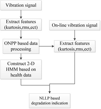
Vibration is one of the most widely used measurements for diagnostics. Thus, when the vibration signal is obtained, the general features can be computed. Since the general features extracted from original signal contain lots of noises which could cause the indicator to show huge randomness, the first step to build NLLP based degradation indicator is to use ONPP for the pretreatment of the high-dimensional data composed of multiple general features extracted from original signal. In the ONPP based pretreatment, the low dimensional number selected for the construction of indicator is determined according to experience, which sometimes is 2-4. Then, the new low-dimensional health data is used to train 2-D HMM which can represent the characteristic of the health condition. Afterwards, NLLP based index can be utilized for the assessment of the degradation performance when the on-line data is obtained. The data that need to be monitored should be also processed by ONPP to eliminate the negative effects of the noise. Then the negative log likelihood probability can be computed using the 2-D HMM model trained by the health data, which indicates the degree that the monitoring data deviated from the health condition. If the value of negative log likelihood probability is bigger, it indicates the degree that the data deviated from the health condition is bigger. Thus, it can tell that something abnormal may happen. The construction procedure of NLLP based index is shown in Fig. 1.

Fig. 1System framework for bearing performance degradation assessment

3.1. Experimental data

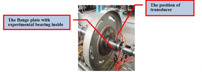
In order to evaluate the effectiveness of the proposed method for degradation performance of rolling elements bearings, several experiments are conducted in this study. The experimental device showed in Fig. 2 consist several main components which are the supporting structure for bearing, transmission shaft, Servo-driven Motor, lubrication system, axial loading device and control system. The experimental bearing type is NSK7010C.

Fig. 2Experimental setup: a) is the integral figure of the experimental device; b) is the partial enlarged detail map of supporting structure for bearing

a)

b)

In order to accelerate the fatigue, the experimental bearing whose rated axial load is 13.9 kN is working under the high strength operating condition with the axial load 20 kN. The measuring instrument is B&K3560C. Two sensors are used for data collection. One sensor is located on the outside flange while another one is located on the chassis. Four bearings are used in this experiment and every bearing is under the same work condition. The experiment begins as the engine is started. In the experimental process, the computer connecting to the measuring instruments is used for monitoring the vibration amplitude. Once the amplitude becomes large the experiment ends. Then the next bearing can be mounted in the test rig for experiment. The experimental rotating speed is 4000 rm/min, and the sampling frequency is 65536 Hz. Every sampling length of the data segment is 20 s, and the interval of the data segment is 10 min. Four groups of data are used for degradation performance evaluation in this paper.

Fig. 3The kurtosis map of the full life

Fig. 4The RMS map of the full life

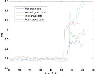
Fig. 5The skew map of the full life

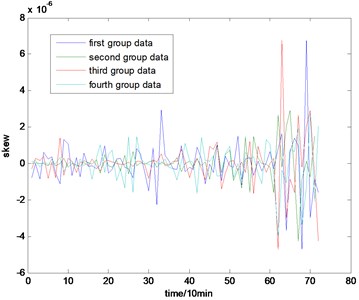
Fig. 6The peak map of the full life

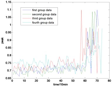
The selection of the general fault features is in accordance with experience. In this paper, four kinds of general fault features are used for condition monitoring, which are kurtosis, root mean square (rms) value, skew, and peak value. The whole life cycle maps of the four groups of data are shown in Figs. 3, 4, 5, and 6. The corresponding equations are shown as follow:

$X$ is the data segment while $N$ is the corresponding length. $s$ is the variance. $k_3$ and $k_2^{}$ respectively represent third and two order central moment.

3.2. The data processing based on ONPP

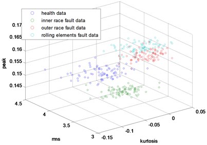
In this part, the general features will be preprocessed by ONPP, and the eigenvectors with relevant eigenvalues will be obtained. Then we choose several eigenvectors corresponding to the smallest eigenvalues to compute the new low dimensional data as the output, and the number of the eigenvectors selected equals to the dimensional number of the new data. Since two and three-dimensional data distribution of the bearing defect classes can be visualized well in this experiment, we select two and three-dimensional data to construct effect figures which are shown in Fig. 7 and Fig. 10. Fig. 7 is the two-dimensional figure processed by ONPP while Fig. 10 is the three-dimensional figure processed by ONPP. Several general features are used to construct the two-dimensional and three-dimensional figures for comparison, which is shown in Figs. 8, 9, 11, and 12. As can be seen in Fig. 7 and Fig. 10, the fault classification processed by ONPP is clear whether the first two or three principle elements are chosen. However, the general features based fault classification totally can’t be distinguished, which are shown in Figs. 8, 9, 11, and 12. Therefore, the data processed by ONPP is more effective for fault classification in comparison to the general features.

Fig. 7The distribution map of data processed by ONPP with two features

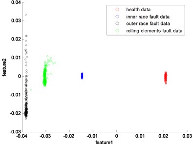
Fig. 8The distribution map of kurtosis and rms

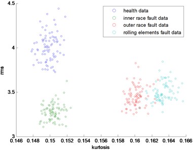
Fig. 9The distribution map of kurtosis and skew

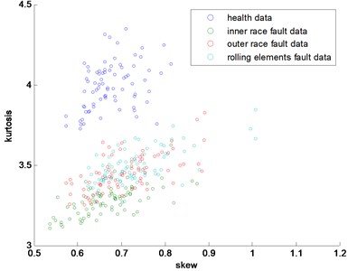
Fig. 10The 3-dimensional distribution map of data processed by ONPP with three features

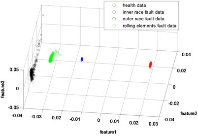
Fig. 11The 3-dimensional distribution map of skew, kurtosis and rms

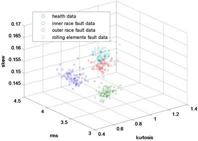
Fig. 12The 3-dimensional distribution map of skew, peak and rms

3.3. The analysis of the 2-D HMM based NLLP indicator

A quantification degradation indication can increase the effectiveness of residual life prediction of key machine components. In this part, the new low dimensional data is used for the construction of degradation indicator. The health data is needed for training due to degradation trend of these general fault features. In the figures of these general fault features, the variation tendency of first 20 data points change little and thus the first 20 sample of the processed data can be used for training. The states number of 2-D HMM have little impact on the model, and little applicable method can be utilized for the option of the states number. In application areas of 2-D HMM, the states number is generally below 10 according to the experience. Therefore, 5 simple-states and super-states are chosen to build the 2-D HMM. Since the states of the 2-D HMM do not express practical sense, the initial state distribution and the state transmission matrix can be randomly selected. In order to better train the model, the parameters within the Gaussian mixture function of the 2-D HMM, which are mean, variance, and weights, can be initialized by some clustering algorithms.

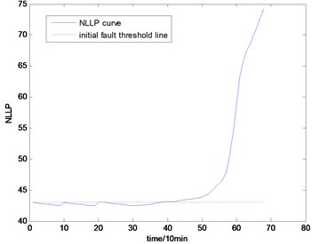
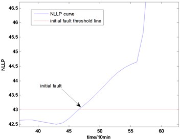
Fig. 13The NLLP indicator map of the first group of data: b) is partial enlarged detail map of a)

a)

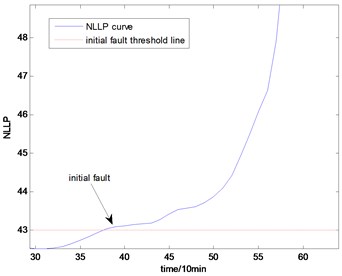
b)

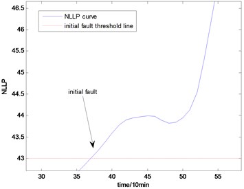
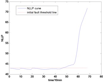
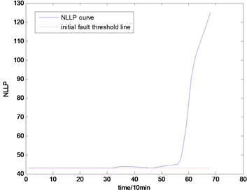
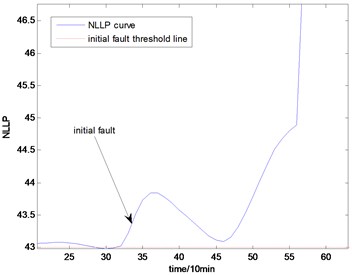
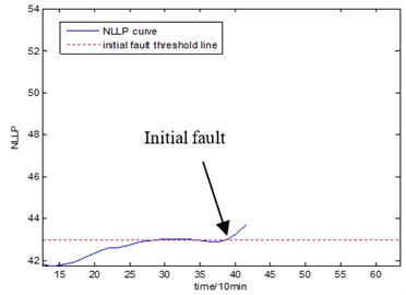
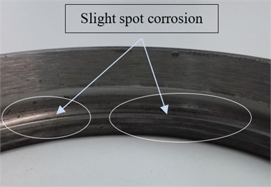
With the health data based 2-D HMM trained, the proposed indicator can be made, which is shown in Figs. 13-16. As is shown in these figures, little change can be seen in the first 35 samples which can be regard as the health condition. Then 35 samples later, the degradation tendency present a significant increase compared with the whole life cycle maps of the general features. In Fig. 13, the slight degradation increase can be observed after the 38th data point. From the Fig. 13 to Fig. 16, the same results can also be noticed. But in Figs. 3-6, which show the trend of the general features based indicator, little distinct degradation with a sudden change is shown. Although the kurtosis and RMS can show the implicit fault moment at about the 50th data point in comparison to other general features, they are still far short of the proposed indicator. Otherwise, the tendency of the proposed index is slippery and presents less noise. Briefly, the proposed index can present better degradation trend and more apparent weak-defect compared with the general features. From these figures, the weak-defect threshold can also be chosen in terms of the red line at around 43. Therefore, the proposed indicator is more effective than the indicator based the general features. An extra experiment is added to validate the occurrence of the initial fault which truly happened as the revealing of proposed indicator. As is shown in Fig. 17, we take out the bearing from the test rig at the 42th sample in Fig. 17(a), and slight spot corrosion happening in outer race can be seen in Fig. 17(b).

Fig. 14The NLLP indicator map of the second group of data: b) is partial enlarged detail map of a)

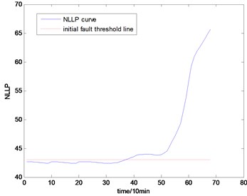
a)

b)

Fig. 15The NLLP indicator map of the third group of data: b) is partial enlarged detail map of a)

a)

b)

Fig. 16the NLLP indicator map of the fourth group of data: b) is partial enlarged detail map of a)

a)

b)

Fig. 17Initial fault map

a)

b)