Abstract
Determination of general parameters is one of the most essential tasks in optimal structural designs to increase firing accuracy or firing stability, since they are two of the most important performance requirements in artillery designs. This paper presents a multi-objective optimization approach, based on multidisciplinary agent model method. An experiment verified artillery multi-body rigid-flexible coupled dynamic model was first presented. Sample library was generated by optimal Latin hypercube design algorithm and this dynamic model. Then a radial basis function-back propagation neural (RBF-BP series combine) network model was developed to predict firing parameters, used the sample library to train and test the validation of developed neural network model. Finally, an application case was given by NSGA-II and the max-min criterion, its results demonstrate the effectiveness of our method through comparing with its original value.
1. Introduction and literature review
The firing process of towed artillery is with huge transient impact load, it is a strong nonlinear vibration problem. As one of the most important tactical and technical properties in weapon design, firing accuracy plays a key role in artillery design and evaluation. Also, firing stability attracts more and more attentions in artillery researches with the improvement of the firing range and the increase of its power, especially in large caliber artillery.
In system design stage, weapon designers concern a lot on how to reasonably allocate artillery structure and dynamics parameters to improve firing accuracy or stability [1], which are belong to the category of vibration control and vibrostabilization respectively. Fan C. J. [2] analyzed the influence of tube bending on firing accuracy. Zhou L. et al. [3] optimized recoil resistances and muzzle disturbance by ADAMS basic development module and niche genetic algorithm. Sava A. C. et al. [4] presented a method of recording the flexural vibrations of the barrel and analyzed its influence on the firing accuracy. Wang R. L. et al. [5] proposed a concept of dynamic stability, they considered gun firing stability as to make the transient fire units of every projectile came out of muzzle have a good consistency, in other words which is to keep them in a permitted range. Yu Z. P. et al. [6] used a genetic algorithm and optimized construction and dynamics parameters of the gun system and its firing stability. Based on the virtual prototype, Chen M. et al. [7] did a research on influences of the structure parameters and the boundary condition on firing stability. Nevertheless, firing accuracy and firing stability are rarely considered together. Actually, they may conflict in some parameters.
For current artillery structure optimization, most of them consider that a list of predefined and pre-evaluated alternative variants of the artillery options is given. In case a small number of such solutions have been defined, there is no guarantee that the solution finally reached is the best one. During the development of modern design technologies and methods, a multi-objective optimization approach is required in order to address all of the above aspects and to find an appropriate tradeoff between the computing efficiency and the complex design parameters requirement [8].
Surrogate model is a kind of design optimization method contains many contents such ad experiment design method and the approximate modeling. It has been widely applicable in many engineering fields [9-11], but these kind of literature were seen rarely in the field of artillery. Cui K. B. et al. [12] calculated the muzzle disturbance, established the nonlinear mapping relationship between the muzzle disturbance and the structure parameters by homogeneous experimental design and radial basis function (RBF) artificial neural network (ANN). Liang C. J. et al. [13] optimized muzzle disturbances of an artillery with a (back propagation) BP neural network, genetic algorithm and finite element method. BP network has the shortage of a slow learning speed, easily falling into the local optimum, the RBF network has fast learning speed and can avoid falling into the most superior advantages, but the training sample dependence is strong, it has poor generalization ability [14].
In our work, a combination of RBF neural network and BP neural network was adopted, which combined with the advantages of both neural network, to improve the generalization performance of the neural network and overcome the standard error of the training sample set. What’s more, firing accuracy and firing stability are simultaneously considering as the optimization objectives. Thus, it will be better to evaluate the artillery performance properties. NSGA-II genetic algorithm and the max-min criterion were selected as the optimization tools which can solve the above drawbacks well.
2. Multi-body rigid-flexible dynamic modeling and model verification
2.1. Multi-body rigid-flexible dynamic modeling
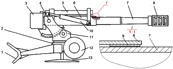
Fig. 1 shows a diagram of the towed artillery. When it is firing the gunpowder combustion produces a large number of high pressure gas, which promotes the projectile a forward movement along the gun bore with a great acceleration. At the same time the recoiling parts, which including the breechblock, recoil mechanism, barrel and muzzle brake, make a backward recoiling and then forward counter recoiling motion under the joint action of the forces of the gun bore and recoil resistance.
Fig. 1Diagram of firepower part of a towed artillery: 1 – spade, 2 – undercarriage, 3 – breechblock, 4 – trunnion, 5 – recoil mechanism, 6 – cradle, 7 – barrel, 8 – muzzle brake, 9 – front bushing, 10 –balancer, 11 – top carriage, 12 – running wheel, 13 – base
Basic hypothesis: regardless of the coupling effect between projectile and barrel in the process of firing. And the artillery was in static equilibrium position before firing.
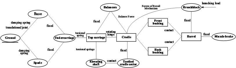
The flexible parts, such as the barrel, cradle and top carriage, were created based on finite element modal neutral file. Their dynamic response was calculated by using the superposition method. The rest parts, which did not affect artillery dynamic response much, were established as rigid parts. Then proper joint relationship and boundary condition was set up between all the parts and the ground. The launching load and forces of recoil mechanism were written in FORTRAN program as a dynamic link library for ADAMS. The topological structure of this dynamic model is presented as Fig. 2.
Fig. 2Topological structure of the dynamic model
2.2. Model verification
In order to verify the artillery launching dynamics model, a series of dynamic verification tests were performed. Usually, there are two aspects need to verify. The first one, testing the recoil displacement and recoil resistance to inspect the rationality of the modeling process and artillery recoil movement. The second aspect, measuring the values of firing dynamic parameters like the angular displacement of the muzzle to evaluate the tactical level of the artillery.
As showed in Fig. 3, a high-speed photography test system was put in place to measure the recoil movement of the towed artillery when firing. It is mainly composed of a high-speed camera, optical lens, a fixed bracket, a computer and an image tracking processing software, and other parts. The Phantom V710 high-speed camera has a wide shooting frequency range, from 6,000 fps to 1,400,000 fps, its minimum exposure duration is 1 us. Optical lens is adopting the Nikkor AF-S 400 mm f/2.8D ED lens. Image tracking software using ProAnalyst software developed by company Xcitex. This test system can catch the white-on-black test marking (showed in Fig. 3) precisely in the whole firing process. Thus, we can get kinematic characteristics of the launching artillery system.
As showed in Fig. 4, a testing device for muzzle dynamic response was set. It is mainly composed of a SDI-ARG-720 angular rate gyroscope and a DEWETRON 1201 data acquisition system.
Fig. 3High-speed photography test system
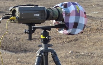
Fig. 4The muzzle responses test
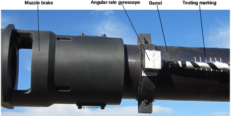
Table 1Simulation and test results
(mm) | (kN) | (deg) | |
Simulation values | 1314 | 420.25 | –0.0152 |
Average testing values | 1281 | 431.62 | –0.0147 |
Relative error | 2.58 % | 2.63 % | 3.40 % |
10 groups firing test were conducted, but 2 of them were get rid since incorrect collecting data. By comparison between the simulation results and the average of 8 groups testing results in Table 1. The less relative error proves the multi-body rigid-flexible coupling dynamic model can simulate the fire process well. Where, is the recoil stroke length, is the maxmum of the recoil resistance, and is the elevation jump angle at muzzle center.
3. Construction of the surrogate model
3.1. Optimization objectives and design variables
Considering the artillery tactical and technical requirements especially for firing accuracy and firing stability, some of the firing dynamic parameters, whose dynamic responses can be used to represent the artillery firing tactical and technical properties, were selected as optimization objectives. The elevation and lateral jump angles at muzzle center, the horizontal displacement of the spade and the vertical displacement of base are included. For all the above parameters, we considered their values at the moment when the projectile came out of the muzzle.
In the multi-body rigid-flexible model of the towed artillery, direct structural sensitivity analysis for flexible parties is not easy because it is difficult to parametric modeling for them which are based on the modal neutral file from FEA. So, we used the related multi-rigid body model to do structural sensitivity analysis, then picked five design variables according to the analysis results and special design requirements. They are the vertical and lateral spectral centroid shift, of recoiling parts, the front cradle bushing’s axial direction offset , the trunnion center’s vertical offset and the gap between cradle bushing and barrel. Where, , and are three of the most important general parameters for artillery designs, and also play the key roles in firing accuracy and firing stability.
The initial values and value ranges of design variables are presented as Table 2. The initial values come from the original design of this towed artillery, and we determine value ranges of design variables by comprehensive considering expert system and design experience in the past years.
Table 2Initial values and value ranges of design variables
Design variables | (mm) | (mm) | (mm) | (mm) | (mm) |
Initial values | 6.23 | –2.56 | 0 | 0 | 0.8 |
Upper limit | 18.23 | 3.44 | 200 | 5 | 1.6 |
Lower limit | –5.77 | –8.56 | 0 | –5 | 0.5 |
3.2. Establishment of sample library
The design of experiment is the sampling plan in design variable space. The key question is how we assess the goodness of such designs, considering the number of samples is severely limited by the computational expense of each sample.
In order to reduce the size of the training database while keeping the sample representative, optimal Latin Hypercube Sampling (LHS) is used. LHS is a stratified sampling approach with the restriction that each of the input variables has all portions of its distribution represented by input values, and optimal LHS have been proposed to overcome the potential lack of uniformity of LHS. Based on optimal LHS algorithm, according to the initial values and value ranges of design variables in Table 2, a MATLAB program was implemented to calculate 130 training samples and 15 validate samples for design variables. Partial training samples and validate samples are listed below in Table 3.
Based on the above dynamic model in Section 2, according to the values of training samples above, we modified multi-body coupling model respectively. Every flexible body part was modified by altering its finite element mesh model to regenerate a new modal neutral file according to the sample parameters, and importing it into the dynamics model to replace the original component. Then, we can run dynamics simulation to get the relative sample output values. All in this way, the training sample, test sample input and output values are obtained, the sample library was created.
Table 3Partial training samples and validate samples
No. | (mm) | (mm) | (mm) | (mm) | (mm) | |
Training samples | 1 | 1.75 | 1.86 | 94.95 | –1.77 | 0.533 |
2 | 10.47 | –8.44 | 86.87 | 1.97 | 0.967 | |
3 | 4.90 | –6.50 | 2.02 | 1.06 | 1.144 | |
4 | –3.83 | –0.56 | 183.84 | 0.05 | 1.256 | |
5 | –5.29 | –2.74 | 107.07 | –3.08 | 1.322 | |
… | … | … | … | … | … | |
130 | 14.36 | –6.72 | 38.38 | 2.58 | 0.733 | |
Validate samples | 1 | 2.80 | 0.87 | 14.286 | 4.29 | 1.129 |
2 | 4.52 | 2.58 | 171.429 | 2.14 | 1.443 | |
3 | 1.09 | –4.27 | 28.571 | 0 | 0.500 | |
… | … | … | … | … | … | |
15 | –5.77 | –3.42 | 157.143 | –3.57 | 1.207 |
3.3. RBF-BP series combine artificial neural network
In the surrogate model construction stage, we use systematic parameter variation and a selection process that takes into consideration both accuracy and architectural simplicity to find and train the most robust surrogate design for each of the considered target variables.
A genetic optimization RBF-BP series combine neural network was built to create the approximate model. It is a series combine neural network with a RBF sub-network and a BP sub-network double hidden layers. According to the related structures of artificial neural network, the output and input relationship equations can be derived by the artificial neural network theory knowledge [15] as below.
The transfer function of the first RBF hidden layer nodes is Gaussian function, it can be written as:
where is a dimensional input vector, is the center of the th radial basis function, and it have the same dimension with , is the width of the th radial basis function of hidden layer neurons, represents the Euclidean norm between and , with the increase of it, will gradually decay till 0. The number of hidden layer neurons in RBF sub-network set as , then the output of the th neurons in the RBF sub-network follows that:
where presents threshold value of the th neurons in RBF sub-network, (1, 2, …, ) presents the weight from hidden layer to output layer of the RBF sub-network. The input of the th neurons in BP sub-network is the sum of the threshold value and the related weighted of the output in all the neurons in RBF sub-network, that is:
where presents threshold value of the th neurons in BP sub-network. The transfer function of the BP sub-network is Tansig-type function, it can be written as:
So, the output of the th neurons in BP sub-network:
Then the output of the th neurons in RBF-BP series combine network is the sum of the threshold value and the related weighted of the output in all the neurons in BP network, that is:
where presents threshold value of the th neurons of output layer in RBF-BP series combine network. For the given sample input () and expected output (), the output error is defined as .
In this manuscript, the RBF-BP series combine neural network structure is five inputs, four outputs and two hidden layers, the number of hidden layer neurons has the approximate relationship with the number l of neurons in the input layer, which is , that is 11. But in order to get a good precision, trial method was used to define the number of the two hidden layer neurons from 9 to 20, and found that when the first and second hidden layer neurons was 15, 15 respectively, a total of 154 weights and 34 thresholds can get better approximating precisions.
The data were initially pre-processed to remove outliers. Additional inputs were formed by means of aggregating operators. The input and output variables were rescaled in the [0.1, 0.9] range to facilitate ANN training. After normalization of the input sample , first training through sub-RBF neural network, the training results as input to the training of BP sub-network, and finally get the training results. And the network has the ability of error back to study, when the training results cannot meet the precision demand, reverse changes of the neural network weights and threshold until the training results meet the accuracy requirements, finally finished the training.
3.4. Validation of surrogate model
When surrogate model constructed, precision evaluations must pass to ensure the validity of the model. The evaluation includes two aspects: the reappearance of sample points and prediction ability of non-samples space points. Here we taken the most commonly validation method, the coefficient of determination , to test this surrogate model. The expression presented below:
where , and are dynamic simulation value (true value) of the th test sample, predicted approximate value by RBF-BP series combine network of the th test sample and the mean value of all the dynamic simulation values of the test samples. is the number of the test samples.
The more of the close to 1, means the more precision of surrogate model. An of 1 means the dependent variables can be predicted without error from the independent variables.
In the process of practical validation on surrogate model, it is usually randomly generated the additional test points in the design for model precision reason. Thus, we use the additional 15 test samples and its dynamic simulation response mentioned in Section 3.3.2 to evaluate the constructed RBF-BP series combine ANN surrogate model. The inspection results show in Table 4. According to that, it can be regarded the established approximate model have a good generalization ability and high prediction accuracy.
Table 4Inspection results
Evaluation criteria | ||||
0.987 | 0.999 | 0.995 | 0.989 |
4. Surrogated-based multi-objective optimization
4.1. Multi-objective optimization
In MO optimization problems, several conflicting objective functions have to be minimized concurrently. Specifically, in our towed artillery optimization, the elevation jump angle and lateral jump angle at muzzle center, the horizontal displacement of the spade and the vertical displacement of the base are selected as the optimization objectives. The first two are responsible for firing accuracy and the rest two are for firing stability. We considered their values in the moment of the projectile came out of the muzzle. They can be illustrated below:
where, are the design variables, their initial value and value range are mentioned in Table 2 previously. , , and are the experience weight coefficients in the evaluation of firing accuracy and firing stability by certain evaluation criterions, here we selected as 0.6, 0.4, 0.3 and 0.7 respectively. , , and are the initial objective value in the original design. And , are the lower limit and upper limit of the design variables , which were also presented in Table 2.
One of the most appropriate strategies to determine a good approximate solution of a NP-hard multi-objective problem is a metaheuristic algorithm based on population which evolves along the solution space to find a set of non-dominated solutions. In this paper, we propose a methodology based on the non-dominated sorting genetic algorithm-II (NSGA-II) first introduced by Deb K. [16]. The main objective of algorithm NSGA-II is to find a set of solutions ordered by fronts under the concept of Pareto dominance.
In our work, the proposed algorithm has been implemented in MATLAB, the parameters used for the proposed algorithm are: the rate of recombination is 95 %, the number of iterations is 300, and the size of the initial population is 80. Once we have an efficient ANN and a well-set NSGA-II algorithm, we can perform the optimization. Fig. 5 shows the Pareto fronts found by the proposed methodology, it offers a range of possibilities depending on the objectives for the proposed problem. In this case, the best solution depends on the specific interests of the decision maker. He would pick solutions close to side A, if pay more attention to firing accuracy, or close to side D for firing stability.
The first part (A to B) and the second part (B to C) are almost linear with a persistent fall of for lower values of , but the slope of the Pareto front is greater for the first part than the second. Indeed, in the first part, the most appropriate axial direction offset of the front cradle bushing’s () will be the optimal solution. But in the second part, it just has little influence on both optimization objectives. And lateral spectral centroid shift of recoiling parts) and the trunnion center’s vertical offset influence a lot. The third part (C to D) corresponds to a relatively gentle fall of for higher values of .
Table 5 indicates that the change of optimization objectives really due to the five design variables, but and are conflicting, they have different change trends. Specifically, just in the numerical view, with the decrease of, and , and the increase of and , the firing accuracy () will become poorer but the firing stability () will be better.
When got these values of the design variables, a optimization towed arillery dynamic model can be obtained by modifying the relative parameters. For the changes of the and , usually making a rearrangement of the affix in the breech and a slight change of the mass of the barrel and muzzel brake can reach the goals. For , and , we need to modify the structure dimensions of the cradle and its related adjacent parts, and all these dimension modifications is easy to do. And in flexible multi-body dynamic modeling level, just as description in Section 3.2, we can modify the finite elements models to change the modal neutral files of the related components and parts. In this way a optimization towed arillery dynamic model can be obtained.
Fig. 5Optimal Pareto front
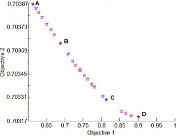
Table 5Values associated to the points A, B, C, and D in Fig. 5
(mm) | (mm) | (mm) | (mm) | (mm) | |||
A | –1.156 | –1.200 | 0.921 | 1.918 | 1.600 | 0.6139 | 0.70386 |
B | –3.770 | –0.220 | 78.037 | 0.384 | 1.492 | 0.6889 | 0.70365 |
C | –4.864 | –0.124 | 71.752 | –0.782 | 1.332 | 0.8138 | 0.70331 |
D | –5.308 | 0.126 | 91.61 | –1.193 | 1.227 | 0.9017 | 0.70317 |
4.2. Selecting a solution of the Pareto front
We got a range of possible optimization results above, and the decision maker can choose a best one for their specific interests. However, there are different ways to select the optimum solution Pareto front.
Max-min criterion is used to select a solution from the Pareto front, in order to show solutions that represent each set of data. This method finds a solution that is equidistant from the ends of each objective. The criterion is defined as follows:
where , are the maximum and minimum values of the objective function 1, , are the maximum and minimum values of the objective function 2, and , are the values of the objective function 1 and function 2 for solution respectively.
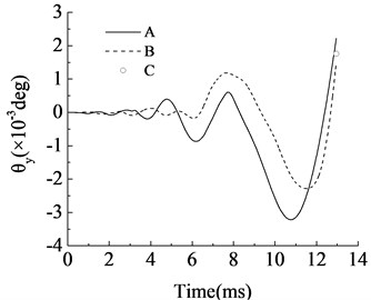
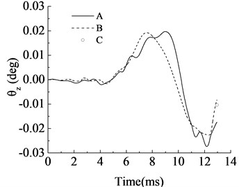
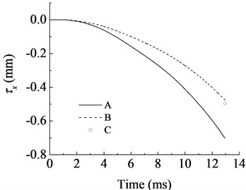
This criterion selects from the Pareto front a specific solution (enclosed in box in Fig. 5), whose characteristic and their relative objectives are shown in Table 5. And the comparisons of optimization objectives between the selected solution and the original design are also showed in Table 7 and Fig. 6.
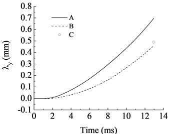
It should be pointed out that our surrogate model only can calculate the parameter values at the moment when the projectile came out of the muzzle, so in the Table 7, we compare the parameter values at that moment in different conditions. While in the Fig. 6, we compare the different parameter values at whole period from firing second to the projectile came out of the muzzle moment, so the selected solution value in surrogate model showed in Fig. 6 just an instantaneous value which are marked as C. And the curve A and curve B indicate the original solution values in ADAMS model and the selected solution values in ADAMS model, respectively.
Table 6Values associated to Chosen solution of the Pareto front in Fig. 5
(mm) | (mm) | (mm) | (mm) | (mm) | |||
Value | –3.66 | –0.26 | 68.42 | 0.38 | 1.42 | 0.7419 | 0.70346 |
Table 7Comparisons of optimization objectives between the chosen solution and the original design
(deg) | (deg) | (mm) | (mm) | |
Selected solution in surrogate model | 0.00176 | –0.01034 | –0.4953 | 0.4891 |
Selected solution in ADAMS model | 0.00147 | –0.00826 | –0.4760 | 0.4589 |
Original solution in ADAMS model | 0.00225 | –0.01520 | –0.7022 | 0.6961 |
Fig. 6Comparisons of optimization objectives between the selected solution and the original design: A – optimization objectives in original design of ADAMS model, B – optimization objectives in selected solution of ADAMS model, C – optimization objectives in selected solution of surrogate model
a)
b)
c)
d)
4.3. Discussions
According to the artillery system dynamics [17] and artillery design theory [18], , and are three of the most important general parameters for artillery designs, and also play the key roles in firing accuracy and firing stability. To be specific, the vertical and lateral spectral centroid shift , of recoiling parts should be as smaller as possible, and trunnion center’s height plays a very important and complex role in firing accuracy and firing stability since the cradle can be rotate slightly around it when firing, its position has key relation to the movement of the artillery because it’s the position of the turning center of the recoiling parts. Similarly, for the gap between cradle bushing and barrel, it also has complex and important effect on firing accuracy and firing stability, it is a complicated contact/collision problem under dynamic impact loading and a thermal phenomenon, many artillery researchers worked on this but it’s hard to decide it in a different situation. For the distance between front and back bushings, since the acting position of the relative sliding between the recoiling parts and cradle are front and back bushings, so theoretically the larger distance , the smaller vibration of the muzzle, and that means the better firing accuracy, however, when the distance is too long in some way, it will influence the overturning moment of the whole artillery, and then the displacement of the spade and the base, that means worse firing stability. So a proper distance is needed to balance the firing accuracy and firing stability. In our optimization design, the front cradle bushing’s axial direction offset is changed to change the distance lx.
Compare with the parameter values in Table 2 and Table 6, it can be found that in our selected solution the vertical and lateral spectral centroid shift , of recoiling parts became smaller, the distance and the gap became larger slightly. Combine with artillery system dynamics and artillery design theory, it is not difficult to explain and verify our optimization results. Actually, it can be seen from Fig. 6 that at the end of the curves B (present the selected solution) have smaller values compare to curves A (present the original design), and curves B also get smaller maximum value at the whole interior period, that means our selected solution has a better tactical and technical properties.
What’s more, the curves B have the similar growth pattern with curves A, they are all similar to the classical situations like reference [3] and [13], and it offers another perspective on the validity of our ADAMS simulation model. And the optimization objectives (curves A) in selected solution of ADAMS model are very close to whose at the surrogate model (point C), this indicates our RBF-BP series combine neural network surrogate model has strong generalization ability and high prediction accuracy, it can reflect the artillery launch system well. All these indicate our optimization method effective and it can verify our optimization results well.
To conclude on these comparisons, the selected solution considered all the four objectives at the same time, they all meet an optimal results. In this way, we can get a relatively balanced solution. Moreover, these also claimed our methodology’s feasible and effective.
5. Conclusions
In this paper, a RBF-BP series combine neural network model was used to approximate the surrogate model for understanding and predicting the relationship between five of the towed artillery general design parameters and the dynamic responses of artillery muzzle center, the spade and the base, which are the key factors related to artillery firing accuracy and firing stability. In order to optimize the firing accuracy without reducing the firing stability, a methodology was presented by implementing a non-dominated sorting genetic algorithm (NSGA-II), the results show a set of non-dominated solutions organized in a Pareto optimal front, reflecting the conflict between the two considered objectives. Therefore, the proposed approach provides the opportunity to choose any of the solutions of the front according to the criteria chosen by the decision maker. In addition, a criterion for choosing a good quality solution was also proposed. The optimization results showed that both the firing accuracy and firing stability were improved obviously. This confirms that our methodology is feasible and effective.
It is an exploratory study on optimization of flexible parts in rigid-flexible multi-body dynamic system and so as to get an optimization scheme to improve the firing accuracy and firing stability at the same time. Further considerations, such as how to get a more accurate dynamic response, to generate an experimental measurement and analysis combined sample library, and to get a serials of experimental verification of the surrogate model should be included in the future work. Furthermore, the projectile-barrel coupling influence could be explored in dynamic modeling.
References
-
Kathe E. L. Proceedings of the US Army Symposium (9th) on Gun Dynamics Held in McLean, Virginia on 17-19 November 1998. No. ARCCB-SP-99015. Army Armament Research Development and Engineering Center Watervliet Ny Benet Labs, 2000.
-
Fan C. J. Analysis of the Influence of Tube Bending on Cannon Firing Accuracy. Nanjing University of Science and Technology, Nanjing, 2003.
-
Zhou L., Yang G. L., Ge J. L., Wang F. Structural multi-objective optimization of artillery recoil mechanism based on genetic algorithm. Acta Armamentar ii, Vol. 3, 2015, p. 433-436.
-
Sava A. C., Piticari I. L., et al. The analysis of the vibratory movement of the gun barrel and its influence on the firing accuracy. International conference Knowledge-Based Organization, Vol. 21, Issue 3, 2015, p. 883-887.
-
Wang R. L., Chen Y. S., Hao Y. W. Principle and application of dynamical stability of machine guns. Journal of Nanjing University of Science and Technology, Vol. 28, Issue 3, 2004, p. 265-268.
-
Yu Z. P., Qian L. F., Xu Y. D., et al. Firing stability optimization of truck mounted gun system based on dynamic simulation. Journal of Gun Launch and Control, Vol. 3, 2006, p. 36-40.
-
Chen M., Ma J. S., Wang R. L., et al. Research on influence of structure parameters on firing stability of machine gun based on the virtual prototype. Acta Armamentar ii, Vol. 10, 2008, p. 1167-1171.
-
Zăvoianu A. C., Bramerdorfer G., Lughofer E., et al. Hybridization of multi-objective evolutionary algorithms and artificial neural networks for optimizing the performance of electrical drives. Engineering Applications of Artificial Intelligence, Vol. 26, Issue 8, 2013, p. 1781-1794.
-
Wang G. G., Shan S. Review of metamodeling techniques in support of engineering design optimization. Journal of Mechanical Design, Vol. 129, Issue 4, 2007, p. 370-380.
-
Kleijnen J. P. Kriging metamodeling in simulation: a review. European Journal of Operational Research, Vol. 192, Issue 3, 2009, p. 707-716.
-
Long T., Guo X., Peng L., et al. Optimization strategy using dynamic radial basis function metamodel based on trust region. Journal of Mechanical Engineering, Vol. 7, 2014, p. 184-190.
-
Cui K. B., Qin J. Q., Di C. C., et al. Research on establishment measures of artillery objective function by uniform design method and RBF network. Journal of Machine Design, Vol. 2, 2013, p. 45-48.
-
Liang C. J., Yang G. L., Wang X. F. Structural dynamics optimization of gun based on neural networks and genetic algorithms. Acta Armamentar ii, Vol. 5, 2015, p. 789-794.
-
Zhu Z. W., Guo F., Sun G. H., et al. Research on photovoltaic maximum power point tracking based on RBF-BP neural network. Computer Simulation, Vol. 32, Issue 2, 2015, p. 131-134.
-
Simon H. Neural Networks, a Comprehensive Foundation, Second Edition. Prentice Hall, l998.
-
Deb K. Multi-Objective Optimization Using Evolutionary Algorithms. Vol. 16. John Wiley and Sons, Kanpur, 2001.
-
Kang X. Z., Wu S. L., Ma C. M. Gun System Dynamics. National Defense Industry Press, Beijing, 1999.
-
Zhang X. Y., Zheng J. G., Yang J. R. Gun Design Theory. Beijing Institute of Technology Press, Beijing, 2005
Cited by
About this article

This work-related projects are kindly supported by the National 973 Plan (No. 1503613249), National Science Foundation of China (11572158), National Major Scientific Instruments and Equipment Development Projects (2013YQ47076508) and the Fundamental Research Funds for the Central Universities (No. 30915118825). The authors thank all involved partners for their kind supports. This publication reflects only the authors’ views.
