Abstract
To address the non-stationary and nonlinear characteristics of vibration signals produced by rolling bearings and the noise pollution of acquired signals, a fault diagnosis method based on singular value decomposition (SVD), empirical mode decomposition (EMD) and variable predictive model-based class discrimination (VPMCD) is proposed in this paper. VPMCD is a novel pattern recognition method; however, according to the results obtained when the fault diagnosis method is applied to a small sample, the stability of the VPM constructed based on the least squares (LS) method is not sufficient, as demonstrated by the multiple correlations found between independent variables. This paper uses the partial least squares (PLS) method instead of the LS method to estimate the model parameters of VPMCD. Compared with the back-propagation neural network (BP-NN) and least squares support vector machine (LS-SVM) methods, based on numerical examples, the method presented in this paper can effectively identify a faulty rolling bearing.
1. Introduction
Rolling element bearings are significant components of rotary machines, and their working condition can directly affect the operation of the machine. The failure of a bearing can lead to the failure of the entire structure. Therefore, the early fault diagnosis of rolling element bearings can improve the safety of operating machinery [1-3].
The first step in fault diagnosis is to extract fault features from rolling bearing signals. Because the vibration signal carries large amounts of information representing the health conditions of mechanical equipment, vibration analysis has been established as the most common and reliable method of analysis in the field of condition monitoring and diagnostics of rotating machinery. When a fault occurs, the generated vibration signals are mostly nonlinear and non-stationary [3-5]; therefore, the key to bearing fault diagnosis is determining how to extract fault features from nonlinear and non-stationary signals. Conventional signal processing techniques, such as time-domain statistical analysis, Fourier transforms, and Wigner-Viller distributions, are based on the assumption that the signals are stationary and linear, which is not realistic. Wavelet transforms can be used process nonstationary signals. However, energy leakage will occur in the wavelet transformation, and the selection of the wavelet base function in the wavelet transform is difficult. The EMD method is a time-frequency analysis method suited to addressing nonlinear and non-stationary signals and can decompose signals into several stable intrinsic mode function (IMF) components [6, 7]. EMD has been widely applied in the fault diagnosis of rolling element bearings [8-10]. The collected signals are often mixed with noise, which can increase the number of layers of the EMD and enhance end effects, mixing fault feature signals and noise and increasing the difficulty of extracting fault features [10]. Therefore, selecting appropriate de-noising methods to remove the noise signals is very important and improves the accuracy of feature extraction. De-noising methods based on SVD represent effective nonlinear filtering methods with high robustness and are also used in the fields of image processing and signal filtering [11-13]. Entropy can be used to not only represent the complexity of signals but also measure the non-determinacy of a system or a piece of information [1, 14, 15]. When different bearing faults occur, the energy distributions of signals will change in different bands. Therefore, the energy entropy of vibration signals can be used as the eigenvector to extract fault features.
After extracting fault features from vibration signals, many scholars adopt neural networks, support vector machines (SVMs) or other intelligent methods to identify the fault features of bearings [1, 15, 16]. However, neural network identification methods are built based on large training samples. Their training speed is low, and such methods can easily fall into local extrema [17]. SVMs represent a method of small-sample learning that can obtain a globally optimal solution; however, the kernel function and parameters are not easy to confirm. Because the internal relations between the features of different faults obviously differ, the relations can be used to perform fault diagnosis. Thus, a new pattern recognition method based on the VPMCD method was proposed by Raghuraj and Lakshminarayanan [18, 19]. Cheng adopted the VPMCD method to study the fault diagnosis of bearings and to improve diagnosis performance [20]. LS regression is used in the VPMCD method to estimate the model parameters based on the assumption that no highly linear correlations exist between independent parameters. However, the fault feature data are limited in practical situations such that a linear correlation between independent variables is inevitable for small samples. A high degree of correlation influences the accuracy of parameter estimation, therein increasing model error and destabilizing the model. To address this problem, instead of the LS method, PLS regression is used to estimate the model parameters. The PLS method benefits from a strong processing capacity for high-dimensional data and can estimate parameters given a linear dependence between independent variables to improve the estimation accuracy [21].
In this paper, an improved VPMCD method is used for bearing fault diagnosis. First, an SVD de-noising method is adopted to facilitate the filtering of vibration signals. Then, the EMD method is used to decompose the signals into several IMF components. When a fault appears, some useful faulty information can be extracted from the high-frequency bands of vibration signals. The energy entropy of the first several orders of IMF components is selected to construct the fault eigenvector. The PLS method is selected to estimate the VPMCD model parameters, and the prediction model is applied to facilitate bearing fault identification.
2. Feature extraction of bearing faults based on SVD and EMD
2.1. Effect of noise on EMD
The EMD method proposed by Huang et al. in 1998 was found to be remarkably effective in analysing nonlinear and non-stationary signals [6]. The method can decompose any nonlinear, non-stationary signal into several IMF components and a remainder [8, 9]:
where represents the th IMF and represents the remainder.
During EMD, the upper and lower envelopes are obtained via the cubic spline interpolation of extreme points [10]. Because of the uncertainty of whether the endpoints are the extremes, the spline has a fitting error at the endpoints in each IMF. The error continues to spread to the data internally during the decomposition process, which can lead to the IMF losing its original physical meaning and to false IMF components. Because the vibration signals are polluted by various types of noise to some extent, the number of spline interpolations and layers in the EMD increases, gradually accumulating the error caused by the end effect and seriously affecting the quality of the EMD. Moreover, signals that contain no interference by EMD cannot be well separated into IMF components because of the influence of noise; thus, it is extremely difficult to effectively extract fault features from interfered IMF components.
The effect of interference on EMD is presented in the following example. The simulated signal is:
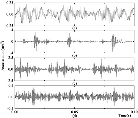
where is the time-domain signal, as shown in Fig. 1, and is a Gaussian white noise signal with an SNR of 14.5 dB. The sampling frequency is 5 kHz, and the sampling duration is 1 s. The IMF components obtained from the EMD are shown in Fig. 2.
Fig. 1Time-domain signal
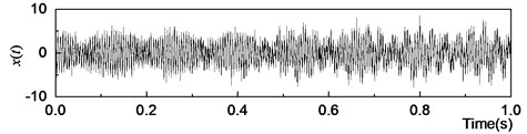
Fig. 2IMF components
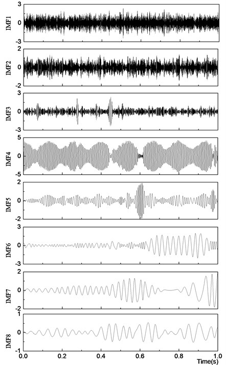
Fig. 2 shows that the 1st-3rd IMF components are mainly noise signals and that the 4th-8th IMF components contain the active ingredient. Due to the influence of noise, frequency aliasing appears in the IMF components. Therefore, the signals containing noise pollution must be preprocessed before applying EMD to improve the accuracy.
2.2. De-noising method based on SVD
The de-noising method based on SVD provides good stability and can reduce noise and improve the SNR [11-13]. Assuming that the vibration signal of a rolling bearing is , the reconstructed track matrix of the attractor is as follows:
According to SVD theory, the matrix is decomposed as , where , , , and . is an diagonal matrix with diagonal elements of , ,…, , which are called the singular values of the matrix , where and . For the signal containing noise, its reconstructed track matrix of the attractor must be a column full-rank matrix, namely, rank . Based on SVD theory and the matrix optimal approximation theorem based on the Frobenius norm, if the first singular values are retained and if the other singular values are set to zero, then the matrix can be obtained via the inverse process of SVD, which is the best approximation matrix of . Thus, the de-noised signals can be obtained from the matrix .
When constructing the best approximation matrix , the de-noising effect differs when the selected order changes. If the order is too low, the information of the filtered signal is not complete, and if the order is too high, the filtered signal continues to contain an excessive noise signal. The singular entropy of the signal can reflect the degree of information contained in the singular value. The singular entropy is defined as follows:
where (1, 2,…, ). Because the first singular value corresponds to the effective components of the signal, the singular entropy is relatively large. After reaching a certain order, the singular value that corresponds to the components of the noise and the singular entropy is relatively small; therefore, the distribution diagram of the singular entropy can be used to determine the order of the effective components. Then, the signal can be reconstructed to effectively and simultaneously retain the signal information and remove the noise. The distribution diagram of the singular entropy is shown in Fig. 3 for the time-domain signal in Fig. 1. The figure shows that after the singular entropy curve decreases to the asymptotic value, the small singular value can be considered as that caused by noise signals. Fig. 3 shows that the order of denoising used to reconstruct the signal is 28.
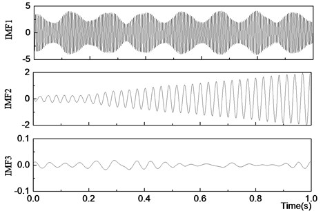
The SNR after de-noising is 55 dB. The first 3 orders of IMF components obtained by EMD from the de-noising signals are shown in Fig. 4.
The figure shows that the de-noising method based on SVD provides good stability and can both reduce noise and improve the SNR. The IMF components obtained from EMD are the effective parts of the signal.
Fig. 3Distribution diagram of singular entropy
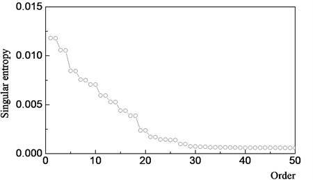
Fig. 4IMF components of filtered signal
2.3. Feature extraction based on energy entropy
When different bearing faults appear, the energy distribution of vibration signals for each order of IMF components changes. Entropy not only represents the complexity of signals but also can be used to measure the uncertainty of a system or a piece of information. Therefore, the distribution of energy characteristics of different IMF components can be described by the energy entropy. For the collected bearing vibration signal , the first orders of IMF components are obtained via EMD; then, the energy , ,…, can be calculated to obtain the energy entropy of each order of IMF components:
where is the proportion of energy of the first orders of the IMF components to the total energy .
3. Improved VPMCD method
3.1. VPMCD method
VPMCD is a novel pattern recognition method that considers linear or nonlinear interrelations among system eigenvalues and assumes that the relations differ in different systems [18, 19]. First, the mathematical models of the interrelations among system eigenvalues are built, and different types of training samples are selected to estimate the model parameters to obtain different predictive models. Then, test samples are identified and classified by the predictive models.
During the bearing fault diagnosis, different eigenvalues are extracted from the vibration signals and are used to describe the characteristics of fault features. There are functional relationships between the eigenvalue and one or more other eigenvalues . In the VPMCD method of this paper, linear interaction VPM is used to establish the interrelations:
where is the order of the predictive model and is the regression parameter of the predictive model.
We use the eigenvalues to predict , that is:
where is the of variable and is the model error.
3.2. VPMCD method based on PLS regression
The VPMCD method based on LS regression (LS-VPMCD) was proposed by Raghuraj et al. to predict the model parameters [18-20]. When the number of samples is small, a linear correlation between independent variables is inevitable. If the linear correlation is strong and if LS regression continues to be used to fit regression models, the regression coefficients will be very sensitive to small changes in sample data; thus, it will be difficult to obtain stable regression models. In practical parameter estimation, multiple correlations between parameters are ubiquitous. Information integration and screening technology are applied when building regression models based on PLS regression. Associations are established with latent factors extracted from predictor variables that maximize the explained variance in the dependent variables, and the noise interference can be excluded to some extent. Thus, this method can effectively solve the regression modelling problem subject to the multiple correlations that exist among independent variables. During bearing fault diagnosis, the model parameters in Eq. (6) are identified as follows [21]:
1) Build the output variable matrix and the input variable matrix using Eq. (6):
where is the number of samples and is the number of input variables.
2) Obtain the normalized variable matrices and as follows, using data standardization to ensure that the collection centre of the sample points coincides with the coordinate origin:
where and are normalized matrices of and , respectively; and are the means of and , respectively; and and are the mean square deviations of and , respectively.
(3) Extract the principal components as follows:
where and . Solve the regression equation of and on as follows:
where and are the regression coefficients and and are the residual matrices.
(4) Replace with , and replace with . Obtain the second principal axis and the second principal components ; then:
Solve the regression equation of and on . Specifically:
(5) Extract the th principal component . Similarly, perform the third step through the th step to obtain principal components , ,…, . The number can be determined via the principle of cross-validation, in which the rank of is less than the rank of .
(6) Reconstruct the PLS regression model. Obtain the PLS regression equation on , ,…, ; thus:
Because , ,…, is a linear combination of , we have:
where . Using Eqs. (18) and (19), we have:
Denoting , , (1, 2,…, ), the standardized regression equation is:
Reconstruct the regression equation of the original variables as follows:
4. A fault diagnosis approach for rolling bearings based on the improved VPMCD method
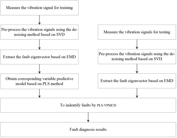
In this paper, SVD, EMD and the PLS-VPMCD are combined to provide fault diagnosis for rolling bearings. Using the SVD method, noise is reduced in the original vibration signals. Then, the EMD method is used to decompose the vibration signals of the rolling bearings into several IMF components. The energy entropy of the first several orders of IMF components is extracted to construct the fault eigenvector, which is combined with the PLS-VPMCD method for pattern recognition. The flow chart of the proposed fault diagnosis approach is shown in Fig. 5.
The fault diagnosis process based on PLS-VPMCD is as follows:
(1) The vibration signals at a certain sample frequency are collected under four types of conditions: the rolling bearing is normal, the bearing has outer race faults, the bearing has inner race faults and the bearing has rolling ball faults. The number of samples is under each condition.
(2) The de-noising method based on SVD is used to pre-process the collected signals, and the reconstruction order is determined by the singular entropy and used to reconstruct the vibration signals.
(3) The EMD method is used to decompose the reconstructed signals to obtain several IMF components. The first orders are selected, and the energy entropy is calculated to construct the fault eigenvector.
(4) The fault eigenvectors under each fault condition are used as the training sample. The corresponding variable predictive model can be obtained using the PLS method as shown in Eqs. (8)-(22), where 1, 2, 3, 4 represent the normal state, the outer race fault state, the inner race fault state and the rolling ball fault state, respectively, and denotes different eigenvalues.
(5) The testing signals are collected, and the eigenvector is constructed according to steps (1)-(3) as the input of the classifier. Then, the working condition and fault classes can be identified by the output of the classifier.
Fig. 5Flow chart of the fault diagnosis model based on PLS-VPMCD
5. Experiment
In this paper, PLS-VPMCD method is used for the fault diagnosis of rolling bearings. Rolling bearing experimental data from the Bearing Data Center of Case Western Reserve University are adopted to verify the validity and superiority of this method. A type 6205-2RS JEM SKF bearing is used. The sampling frequency is 12 kHz, the motor load is 0.746 kW, and the rotational speed is 1797 rpm. The fault types are the normal state, the outer race fault state, the inner race fault state and the rolling ball fault state. The diameter of the fault point is 0.1778 mm, and the depth of the fault is 0.2794 mm. The sampling time of each group is 0.1 s. The acceleration signals of the rolling bearing vibration in the normal state, the outer race fault state, the inner race fault state and the rolling ball fault state are shown in Figs. 6(a)-(d), respectively.
Fig. 6Vibration signal of the rolling bearing
The collected acceleration signal of the rolling bearing vibration is inevitably influenced by noise. In this paper, the SVD method is used to reduce the noise components in the rolling bearing vibration signal. We reconstruct the vibration signals, which correspond to the normal state, the outer race fault state, the inner race fault state and the rolling ball fault state, and calculate the singular entropy of the vibration signal under each working condition, as shown as Fig. 7.
There are different laws for the singular entropy value distribution in each component of a signal. The singular entropy values of the smooth signals and fault signals are larger and mainly appear during the initial period of the singular entropy diagram; thus, the singular entropy value that decreases to the flat region is caused by noise. We select the order for which the singular entropy value decreases to the flat region of the singular entropy curve as the de-noising order. This ensures the validity of the noise filtering process. Fig. 7 shows that the distribution of the singular entropy value exhibits different characteristics during each working state. However, after the 15th order, the singular entropy curve becomes flat; thus, the de-noising order is selected as 15 in this paper. The rolling bearing vibration signals after de-noising in the normal state, the outer race fault state, the inner race fault state and the rolling ball fault states are shown in Figs. 8(a)-(d), respectively.
Comparing Fig. 6 with Fig. 8 shows that the stochastic noise of the signal is largely reduced. The signal after filtering is decomposed using EMD, and the energy entropy of the first 4 orders of the IMF components is used to construct the bearing eigenvector. The first 4 orders of the IMF components decomposed using EMD in the normal state, the outer race fault state, the inner race fault state and the rolling ball fault state are shown in Figs. 9(a)-(d), respectively.
Fig. 7Singular entropy of the vibration signal
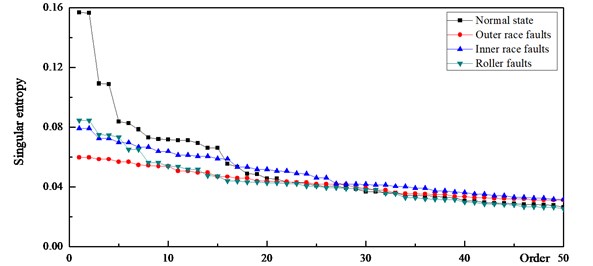
Fig. 8Vibration signal after de-noising
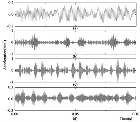
Fig. 9 shows that the SVD de-noising process decreases the influence of noise on the EMD and that each order of the IMF components is the main component of the vibration signal. The characteristics of the energy distributions of the IMF components differ under different fault conditions. The fault eigenvector constructed using the energy entropy of the IMF components can effectively provide information about the bearing work state.
The key point of the VPMCD method used in the fault diagnosis of bearings is obtaining an effective prediction model VPM via training sample regression. With fewer training samples, the number of sample points could be nearly equal to and sometimes less than the number of variables. When the number of samples is smaller, a linear correlation between independent variables is inevitable. If the linear correlation is strong and if LS regression is used to construct the regression model, the accuracy and reliability of the prediction model cannot be easily guaranteed.
The variance inflation factor is the most commonly used diagnostic method when addressing multiple correlations. When the variance inflation factor is larger than 10, multiple correlations strongly influence the estimated value of the LS method. The average variance inflation factors between independent variables are shown in Table 5.
Table 5 shows that the average variance inflation factors between independent variables are much larger than 10. When the model parameters are estimated via the LS method, large deviations appear and subsequently influence the identification precision of the VPM model. The number of samples is 7. VPM models are constructed using the LS method and the PLS method. VPM models are then used to identify 20 new groups of samples, and the VPM model identification errors are shown in Fig. 10.
Fig. 9IMF components of the bearing vibration signal
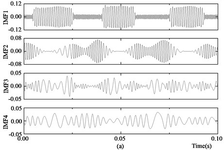
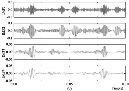
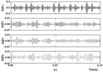
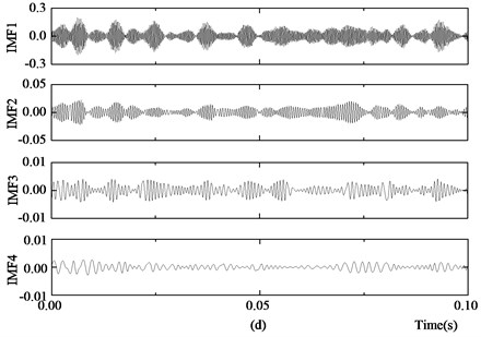
Table 5The average variance inflation factors between independent variables
Dependent variables | Average variance inflation factors | |||
Normal state | Outer race faults | Inner race faults | Roller faults | |
7960.96 | 17742.23 | 7229.62 | 21562.93 | |
2670.89 | 5747.73 | 266007.96 | 13494.77 | |
6012.05 | 3788.70 | 7030.72 | 7015.84 | |
45992.36 | 4704.83 | 3737.37 | 934.01 | |
Fig. 10VPM model identification errors. (VPM1: VPM model constructed using samples in the normal state; VPM2: VPM model constructed using samples in the outer race fault state; VPM3: VPM model constructed using samples in the inner race fault state; VPM4: VPM model constructed using samples in the rolling ball fault state)
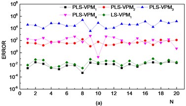
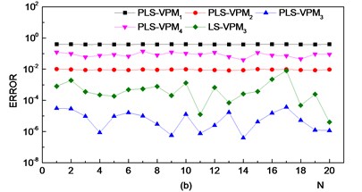
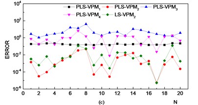
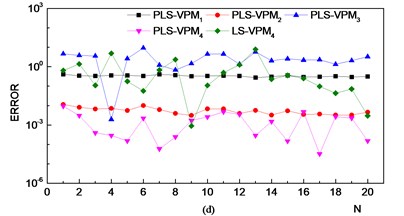
Fig. 11The recognition rates of different methods. A is the recognition rate when the number of samples and when the signal is unfiltered, B is the recognition rate when the number of samples and when the signal is filtered, C is the recognition rate when the number of samples and when the signal is unfiltered, D is the recognition rate when the number of samples and when the signal is filtered, E is the recognition rate when the number of samples and when the signal is unfiltered, and F is the recognition rate when the number of samples and when the signal is filtered
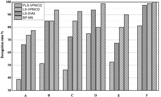
Fig. 10 shows that, because of the multiple correlations amongst independent variables, larger errors appear in the estimated values of the LS-VPM model. Especially for the rolling ball fault state, large errors appear such that it becomes difficult to identify the fault state. The PLS method can effectively solve the problem of multiple correlations amongst independent variables. The error of the estimated value from the PLS-VPM model is stable; thus, the model can properly identify the faulty state of a bearing.
The BP-NN and LS-SVM methods are effective identification methods that possess strong identification abilities and high robustness. Using different numbers of samples when the vibration signals are pre-processed using SVD de-noising and identified using the BP-NN, LS-SVM, LS-VPMCD and PLS-VPMCD methods, the identification error values of 20 new groups of samples are determined, as listed in Table 6. The total recognition rates of 80 groups of samples for different methods are shown in Fig. 11.
Table 6The number of model identification errors
Method | Normal state | |||||
5 | ||||||
Unfiltered | Filtered | Unfiltered | Filtered | Unfiltered | Filtered | |
BP-NN | 12 | 8 | 12 | 4 | 10 | 4 |
LS-SVM | 9 | 2 | 7 | 0 | 9 | 0 |
LS-VPMCD | 2 | 1 | 0 | 0 | 1 | 0 |
PLS-VPMCD | 2 | 1 | 0 | 0 | 0 | 0 |
Method | Outer race faults | |||||
Unfiltered | Filtered | Unfiltered | Filtered | Unfiltered | Filtered | |
BP-NN | 12 | 9 | 10 | 5 | 7 | 2 |
LS-SVM | 5 | 3 | 5 | 3 | 4 | 0 |
LS-VPMCD | 6 | 0 | 4 | 0 | 1 | 0 |
PLS-VPMCD | 5 | 0 | 2 | 0 | 1 | 0 |
Method | Inner race faults | |||||
Unfiltered | Filtered | Unfiltered | Filtered | Unfiltered | Filtered | |
BP-NN | 8 | 7 | 9 | 2 | 9 | 3 |
LS-SVM | 3 | 3 | 0 | 0 | 6 | 0 |
LS-VPMCD | 3 | 1 | 0 | 0 | 0 | 0 |
PLS-VPMCD | 2 | 1 | 0 | 0 | 0 | 0 |
Method | Rolling ball faults | |||||
Unfiltered | Filtered | Unfiltered | Filtered | Unfiltered | Filtered | |
BP-NN | 17 | 15 | 12 | 9 | 12 | 6 |
LS-SVM | 10 | 4 | 10 | 2 | 7 | 2 |
LS-VPMCD | 10 | 10 | 8 | 16 | 14 | 1 |
PLS-VPMCD | 9 | 3 | 4 | 1 | 7 | 0 |
Table 7 shows the number of model identification errors for various orders (10, 15 and 20) of de-noising when the sample number .
The following is demonstrated by the data in Fig. 11, Table 6 and Table 7:
(1) When the number of training samples 5 or 7, independent variables strongly affect each other through the multiple correlations, making the LS-VPM model less stable, especially as shown by the low identification rate of rolling ball bearing faults. The PLS-VPM model effectively avoids the multi-correlation influence between independent variables. Under the different fault state types, the method achieves high identification accuracy.
(2) After de-noising the original vibration signal using SVD, the fault eigenvector extracted from the original vibration signal can provide information about the bearing’s state. Compared with the unfiltered state, the identification accuracy of each method is strongly increased. Increasing the number of samples without performing signal de-noising using the SVD method cannot improve the identification accuracy. Table 7 shows that selecting the 15th order of the de-noising can improve the identification accuracy.
(3) When the number of samples 10, the identification accuracy of the PLS-VPMCD method is 100 % after the signal is filtered. Therefore, the method can accurately identify the fault state of a bearing. The identification accuracy of the PLS-VPMCD method is higher than that of the BP-NN, LS-SVM and LS-VPMCD methods, which are more suitable for identification when using small samples.
Table 7The number of model identification errors for different orders of de-noising
Method | Normal state (7) | |||
Unfiltered | Filtered | |||
10th order | 15th order | 20th order | ||
BP-NN | 12 | 4 | 4 | 6 |
LS-SVM | 7 | 3 | 0 | 0 |
LS-VPMCD | 0 | 1 | 0 | 0 |
PLS-VPMCD | 0 | 1 | 0 | 0 |
Method | Outer race faults ( 7) | |||
Unfiltered | Filtered | |||
10th order | 15th order | 20th order | ||
BP-NN | 10 | 8 | 5 | 5 |
LS-SVM | 5 | 3 | 3 | 2 |
LS-VPMCD | 4 | 1 | 0 | 1 |
PLS-VPMCD | 2 | 2 | 0 | 1 |
Method | Inner race faults ( 7) | |||
Unfiltered | Filtered | |||
10th order | 15th order | 20th order | ||
BP-NN | 9 | 3 | 2 | 2 |
LS-SVM | 0 | 0 | 0 | 0 |
LS-VPMCD | 0 | 0 | 0 | 0 |
PLS-VPMCD | 0 | 0 | 0 | 0 |
Method | Rolling ball faults () | |||
Unfiltered | Filtered | |||
10th order | 15th order | 20th order | ||
BP-NN | 12 | 7 | 9 | 6 |
LS-SVM | 10 | 3 | 2 | 4 |
LS-VPMCD | 8 | 14 | 16 | 12 |
PLS-VPMCD | 4 | 1 | 1 | 2 |
6. Conclusions
A bearing fault diagnosis method based on the SVD de-noising method and the PLS-VPMCD method is proposed in this paper to address the vulnerabilities faced by rolling bearings, the non-stationary and nonlinear characteristics of vibration signals and the presence of noise signals found in the collected signals. The results prove that, when performing fault diagnosis using small samples, the PLS-VPMCD can effectively avoid unstable model parameter identification caused by multiple correlations amongst independent variables. The PLS-VPMCD method achieves a higher diagnostic accuracy than the BP-NN and LS-SVM methods, and the PLS-VPMCD method does not require complicated parameter adjustments, thus avoiding the parameter optimization problem. As a result of the de-noising process using SVD, the fault eigenvector extracted from the original vibration signals can effectively provide fault feature information, reducing the influence of noise on bearing fault diagnosis and improving identification accuracy. Selecting the appropriate order of de-noising can improve the identification accuracy. In this paper, we provide a new analysis method based on PLS-VPMCD for diagnosing ball bearing faults.
References
-
Ben Ali J., Fnaiech N., Saidi L., Chebel-Morello B., Fnaiech F. Application of empirical mode decomposition and artificial neural network for automatic bearing fault diagnosis based on vibration signals. Applied Acoustics, Vol. 89, 2015, p. 16-27.
-
Li Xu, Zheng A’nan, Zhang Xunan, Li Chenchen, Zhang Li Rolling element bearing fault detection using support vector machine with improved ant colony optimization. Measurement, Vol. 46, Issue 8, 2013, p. 2726-2734.
-
Gelman L., Murray B., Patel T. H., Thomson A. Vibration diagnostics of rolling bearings by novel nonlinear non-stationary wavelet bicoherence technology. Engineering Structures, Vol. 80, 2014, p. 514-520.
-
El-Thalji Idriss, Jantunen Erkki A summary of fault modelling and predictive health monitoring of rolling element bearings. Mechanical Systems and Signal Processing, Vols. 60-61, 2015, p. 252-272.
-
Kappaganthu K., Nataraj C. Nonlinear modeling and analysis of a rolling element bearing with a clearance. Communications in Nonlinear Science and Numerical Simulation, Vol. 16, Issue 10, 2011, p. 4134-4145.
-
Huang N. E., Shen Z., Long S. R., Wu M. L., Shih H. H., Zheng Q., Yen N. C., Tung C. C., Liu H. H. The empirical mode decomposition and Hilbert spectrum for nonlinear and non-stationary time series analysis. Proceedings of the Royal Society of London A, Vol. 454, 1998, p. 903-995.
-
Al-Subari K., Al-Baddai S., Tomé A. M., Goldhacker M., Faltermeier R., Lang E. W. EMDLAB: A toolbox for analysis of single-trial EEG dynamics using empirical mode decomposition. Journal of Neuroscience Methods, Vol. 253, 2015, p. 193-205.
-
Dybała Jacek, Zimroz Radosław Rolling bearing diagnosing method based on empirical mode decomposition of machine vibration signal. Applied Acoustics, Vol. 77, 2014, p. 195-203.
-
Georgoulas George, Loutas Theodore, Stylios Chrysostomos D., Kostopoulos Vassilis Bearing fault detection based on hybrid ensemble detector and empirical mode decomposition. Mechanical Systems and Signal Processing, Vol. 41, Issues 1-2, 2013, p. 510-525.
-
Zhang Xiaoyuan, Zhou Jianzhong Multi-fault diagnosis for rolling element bearings based on ensemble empirical mode decomposition and optimized support vector machines. Mechanical Systems and Signal Processing, Vol. 41, Issues 1-2, 2013, p. 127-140.
-
Yang W. X., Tse P. W. Development of an advanced noise reduction method for vibration analysis based on singular value decomposition. NDT&E International, Vol. 36, Issue 6, 2003, p. 419-432.
-
Wee Chong-Yaw, Paramesran Raveendran Measure of image sharpness using eigenvalues. Inform Sciences, Vol. 177, Issue 12, 2007, p. 2533-2552.
-
Jiang Yonghua, Tang Baoping, Qin Yi, Liu Wenyi Feature extraction method of wind turbine based on adaptive Morlet wavelet and SVD. Renewable Energy, Vol. 36, Issue 8, 2011, p. 2146-2153.
-
Huang Jian, Hu Xiaoguang, Geng Xin An intelligent fault diagnosis method of high voltage circuit breaker based on improved EMD energy entropy and multi-class support vector machine. Electric Power Systems Research, Vol. 8, Issue 2, 2011, p. 400-407.
-
Yang Yu, Yu Dejie, Cheng Junsheng A roller bearing fault diagnosis method based on EMD energy entropy and ANN. Journal of Sound and Vibration, Vol. 294, Issues 1-2, 2006, p. 269-277.
-
Fernández-Francos D., Martínez-Rego D., Fontenla-Romero O., Alonso-Betanzos A. Automatic bearing fault diagnosis based on one-class v-SVM. Computers and Industrial Engineering, Vol. 64, Issue 1, 2013, p. 357-365.
-
Liu Zhiwen, Cao Hongrui, Chen Xuefeng, He Zhengjia, Shen Zhongjie Multi-fault classification based on wavelet SVM with PSO algorithm to analyze vibration signals from rolling element bearings. Neurocomputing, Vol. 99, 2013, p. 399-410.
-
Rao Raghuraj, Samavedham Lakshminarayanan VPMCD: Variable interaction modeling approach for class discrimination in biological systems. Febs Letters, Vol. 581, Issue 5, 2007, p. 826-830.
-
Rao Raghuraj, Samavedham Lakshminarayanan Variable predictive models – a new multivariate classification approach for pattern recognition applications. Patten Recognition, Vol. 42, Issue 1, 2009, p. 7-16.
-
Yang Yu, Wang Huanhuan, Cheng Junsheng, Zhang Kang A fault diagnosis approach for roller bearing based on VPMCD under variable speed condition. Measurement, Vol. 46, Issue 8, 2013, p. 2306-2312.
-
Carlos Gérson De Paulo, Pedrini Helio, Schwartz William Robson Classification schemes based on Partial Least Squares for face identification. Journal of Visual Communication and Image Representation, Vol. 32, 2015, p. 170-179.
Cited by
About this article

