Abstract
Aiming at the disadvantage that multi-scale entropy only analyzes the low-frequency components of time series, this paper proposes a rolling bearing fault feature extraction method based on hierarchical dispersion entropy (HDE). Firstly, the HDE is constructed based on the hierarchical operators and dispersion entropy. Secondly, the influence of HDE parameters on entropy stability is studied. Finally, the fault diagnosis method based on HDE, least square support vector machine is applied in rolling bearings. The experiment results show that the proposed method can distinguish different types of the rolling bearing faults. It owns the higher fault diagnosis accuracy than the traditional multi scale entropy methods, such as multi-scale sample entropy (MSE), multi-scale dispersion entropy (MDE).
Highlights
- HDE is used to extract rolling bearing fault features.
- HDE is constructed based on the hierarchical operators and dispersion entropy.
- HDE and LSSVM are applied into rolling bearing fault diagnosis system. It can distinguish different fault types with a higher accuracy than traditional methods.
1. Introduction
As one of the key parts of rotating machinery, the running health of rolling bearing is related to the operation of the whole equipment. It is of great significance to accurately diagnose the fault state of rolling bearing. Due to the complexity of working conditions, fault vibration signals often show non-stationary and nonlinear characteristics [1, 2]. Entropy is an important method to extract features of non-stationary signal. Yan et al. [3] put forward a machine health detection method based approximate entropy. The experiment proves this method owns a nice computational efficiency in the bearing fault diagnosis. Richman et al. [4] proposed sample entropy on the basis of approximate entropy, which overcomes the shortcomings of the approximate entropy self-matching. Yan et al. [5] applied permutation entropy to the feature extraction and condition monitoring of vibration signals. The results show that permutation entropy can detect the dynamic changes of vibration signals of rolling bearings under different conditions. However, approximate entropy, sample entropy and permutation entropy can only measure the complexity of time series on a single scale. Multi-scale entropy own multi dimensional analysis ability and strong stability, so multi-scale entropy can obtain more fault feature information and reflect the complexity characteristics. For this reason, Costa et al. [6] put forward the concept of multi-scale entropy (MSE). Firstly, the time series is segmented on a spatial scale, and then the entropy of samples under each scale are calculated. The complexity of time series at different scales is obtained. For this reason, more information can be analyzed by introducing multi-scale entropy. Zheng et al. [7] designed a fault diagnosis method of rolling bearing based on the multi-scale permutation entropy, which is applied to the fault feature extraction and diagnosis of rolling bearing. The effectiveness and superiority of the proposed method are verified by the comparison results. However, the multi-scale entropy only considers the low-frequency component of the original sequence and ignores the high-frequency component. For the rolling bearing time series with rich fault information distribution, the multi-scale entropy can't meet the requirements [8]. In order to extract the fault information of high-frequency components in the signal, Jiang et al. [9] introduced the concept of hierarchical entropy. Compared with multi-scale entropy, hierarchical entropy considers both low-frequency components and high-frequency components in the signal, so as to provide more comprehensive and accurate time mode information [10]. Azami et al. [11, 12] proposed dispersion entropy to alleviate the shortcomings of sample entropy. Compared with sample entropy, discrete entropy solves the problem of abrupt change in similarity measurement of sample entropy. Moreover, dispersion entropy has the advantages of simple and fast calculation [13-15]. Therefore, on the basis of hierarchical entropy and dispersion entropy, this paper proposes a rolling bearing fault diagnosis method based on HDE. This method can consider the high-frequency and low-frequency components of rolling bearing, and can comprehensively and accurately reflect the working state information of rolling bearing.
This paper is organized as follows: Selection 2 proposes HDE. Section 3 studies parameters selection of HDE method. Section 4 analyzes the classification results of LSSVM [16] based on HDE as well as the comparison results with other methods. Finally, Section 5 concludes this research.
2. HDE method
Based on the advantages of hierarchical entropy and the definition of dispersion entropy, HDE is proposed. The calculation process of HDE is presented as follows:
1) Given the time series , the hierarchical operator and is defined as:
where is a positive integer, the length of the operator and the operator is . According to the operator and , the original sequence can be reconstructed as:
When or , one can define the matrix operator as:
(2) Construct a dimension vector , then the integer can be expressed as , where the vector corresponding to a positive integer .
(3) Based on the vector , the node component of each layer decomposition of the time series is defined as:
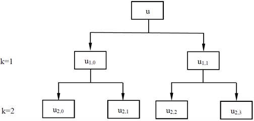
and are the low-frequency and high-frequency parts of the original time series in the layer , respectively. In Fig. 1, the hierarchical decomposition on the scale 2 is illustrated in the form of hierarchical tree.
Fig. 1Hierarchical decomposition with two layers
(4) The hierarchical component sequence is mapped to by the normal cumulative distribution function . locates in the interval .
(5) is assigned to the integer by the function . is the number of categories. is converted to the reconstruction sequence based on the embedding dimension and delay parameter :
(6) All possible discrete models are constructed by using the embedding dimension and class categories .
(7) is matched with discrete models one by one. Then, Eq. (6) is used to count the frequency of each discrete model in the reconstruction sequence :
7) Based on the definition of information entropy, the single dispersion entropy is:
Finally, the HDE can be expressed as:
3. The parameters selection of HDE method
According to the definition of HDE, five parameters need to be set before calculating HDE. Signal length , embedding dimension , number of classes , time delay and number of decomposition layers . When is too large, it will affect the calculation efficiency and reduce the points participating in the calculation of each hierarchical component. Otherwise, when the value is too small, the frequency band division of the original sequence is not detailed enough to obtain enough hierarchical components from low frequency to high frequency. For these reasons, this paper sets . In Generally, time delay is set 1 to preserve the integrity of feature information in HDE. In order to evaluate the sensitivity of HDE to signal length , this paper calculates the HDE entropy and of 50 groups of white noise and 1/ noise with different length. By calculating the mean and standard deviation at different levels, the degree of node dispersion is judged by coefficient of variation (CV). The coefficient of variation CV is equal to standard deviation / mean. As shown in Fig. 2, the larger the signal length , the higher the stability, and the smaller the error bar. The gap between 1024 and 4096 is no longer obvious. It can be seen from table 1 that the larger the signal length, the smaller the CV value, and the more stable the calculation of HDE. This paper selects the best signal length 1024.
Fig. 2Effect of Signal length Non HDE
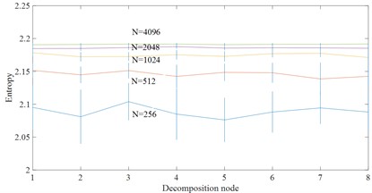
a) White noise
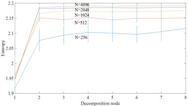
b) 1/ noise
Table 1CV values of node 4 for different signal lengths
Signal length | 256 | 512 | 1024 | 2048 | 4096 |
White noise | 0.0373 | 0.0164 | 0.0064 | 0.0028 | 0.0013 |
1/ noise | 0.0321 | 0.0134 | 0.0070 | 0.0034 | 0.0018 |
From Table 2 and Fig. 3, the CV value of the embedding dimension 2 is small and it indicates that HDE value has high stability and small error. In this paper, 2 is selected as the best embedding dimension. It can be seen from the CV values of different class numbers in Fig. 4 and Table 3 that the CV value tends to increase with the increase of class number . The coefficient of variation is the smallest and the error rate is the lowest when 3. For this reason, 3 selected as the best class number.
Fig. 3Effect of embedding dimension m on HDE
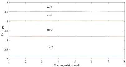
a) White noise
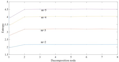
b) 1/ noise
Fig. 4Effect of class number c on HDE
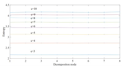
a) White noise
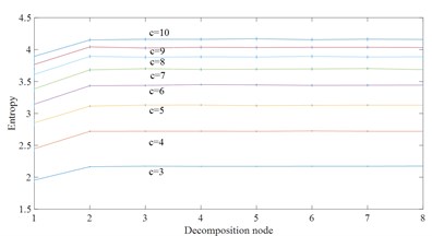
b) 1/ noise
Table 2CV values of node 4 for different embedding dimension
Embedding dimension | 2 | 3 | 4 | 5 |
White noise | 0.0064 | 0.0112 | 0.0174 | 0.0132 |
1/ noise | 0.0070 | 0.0139 | 0.0153 | 0.0119 |
Table 3CV values of node 4 for different classes number c
Class | 3 | 4 | 5 | 6 | 7 | 8 | 9 | 10 |
White noise | 0.0064 | 0.0072 | 0.0101 | 0.0092 | 0.0122 | 0.0132 | 0.0128 | 0.0111 |
1/ noise | 0.0070 | 0.0078 | 0.0084 | 0.0092 | 0.0132 | 0.0123 | 0.0142 | 0.0127 |
4. Experiment
4.1. Introduction to the experiment
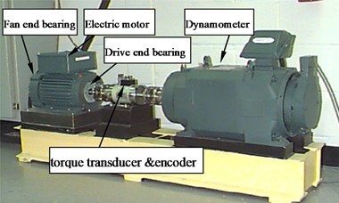
In this section, the feasibility of the proposed method is verified by the fault data of Case Western Reserve University rolling bearing fault test rig. The fault test rig is presented as in Fig. 5. It consists of a 2 hp Reliance Electric motor driving a shaft on which a torque transducer and encoder are mounted. Torque is applied to the shaft via a dynamometer and electronic control system. For the tests, faults ranging in diameter from 0.007 to 0.028 inch, were seeded on the drive- and fan-end bearings (SKF deep-groove ball bearings: 6205-2RS JEM and 6203-2RS JEM, respectively) of the motor using electro discharge machining (EDM). The faults were seeded on the rolling elements and on the inner and outer races, and each faulty bearing was reinstalled separately on the test rig, which was then run at constant speed for motor loads of 0-3 horsepower (approximate motor speeds of 1797-1720 rpm). During each test, acceleration was measured in the vertical direction on the housing of the drive-end bearing (DE), and in some tests acceleration was also measured in the vertical direction on the fan-end bearing housing (FE) and on the motor supporting base plate (BA). The sample rates used were 12 kHz for some tests and 48 kHz for others, Further details regarding the test set-up can be found at the CWRU Bearing Data Center website.
All the vibration data are taken with the sampling frequency 12 kHz. These data include four different health states of rolling bearings, such as inner race fault, outer race fault, ball fault and normal. Each fault state can be divided into four different damage degrees, 0.007, 0.014, 0.021 and 0.028 inch, respectively.
Fig. 5The rolling bearing fault test rig
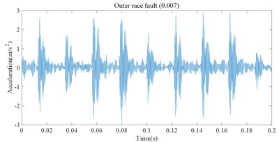
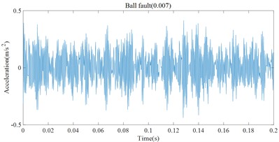
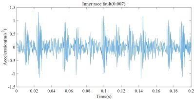
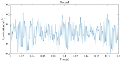
In this paper, the vibration signals of the rolling bearing under 10 fault conditions are collected separately. Such as normal, ball fault(0.007), inner race fault(0.007) ,outer race fault(0.007), ball fault(0.014), inner race fault(0.014), outer race fault(0.014), Ball fault(0.021), inner race fault(0.021), outer race fault(0.021). In this experiment, the vibration signal is divided into multiple data sequences, each of which contains 1024 points. Fig. 6 shows the time domain waveform of bearing fault vibration acceleration signal in this experiment. It can be seen from Fig. 6 that relatively obvious fault impact can occur when there are different fault types of rolling bearing.
Fig. 6The vibration signal of four types of rolling bearings faults
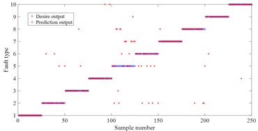
For these fault signal, HDE method is used to estimate the entropy for different fault states. In HDE calculation, embedding dimension 2, number of classes 3, time delay 1 and number of decomposition layers 3. In this feature vector of this experiment, each fault state consists of 50 samples. Each sample includes 8 entropy attributes. Among them, 25 samples of each fault type are randomly selected to form the training sample set (8×250), and the remaining 25 samples formed the test sample set (8×250). This paper utilizes 90 % of cross validation (10-fold Cross validation) estimation. The random experiment is repeated 10 times. Finally, these samples are input into least square support vector machine (LSSVM) [15] back propagation neural network (BP) and naive Bayes classifier (Bayes) so as to realize the intelligent recognition of rolling bearing health status. To verify the superiority of the proposed HDE method, MDE and MSE are also used to extract the rolling bearing fault feature vectors at the same time and input them into LSSVM, BP and Bayes method for pattern recognition. The random experiment is also repeated 10 times. The comparison experiment results are presented in Fig. 7 and Table 4. One can see that the three methods all achieve the best classification results in HDE. For example, for the classification method LSSVM, the average accuracy of HDE is 95.2 %, while the average accuracy of MDE is 88.8 %, and the average accuracy of MSE is 87.2 %. For BP and Bayes, the average accuracy of HDE is the highest compared with MDE and MSE. The main reason is that HDE considers both low-frequency components and high-frequency components in the signal, so as to provide more comprehensive and accurate feature information. But, MDE and MSE only considers the low-frequency component of the original sequence and ignores the high-frequency component [10]. Furthermore, the average accuracy of MDE is the higher than MSE. The main reason is that MDE solves the problem of abrupt change in similarity measurement of MSE [11].
Table 4Comparison of total classification accuracy
Classification algorithm | Classification accuracy | ||||||||
HDE | MDE | MSE | |||||||
Max | Min | Average | Max | Min | Average | Max | Min | Average | |
LSSVM | 96.4 % | 94 % | 95.2 % | 90.4 % | 87.6 % | 88.8 % | 88 % | 86.4 % | 87.2 % |
BP | 88.4 % | 85.2 % | 86.4 % | 80.4 % | 76.8 % | 77.2 % | 76.8 % | 74 % | 74.8 % |
Bayes | 88 % | 84.8 % | 86.8 % | 85.6 % | 83.2 % | 84 % | 84.8 % | 82.8 % | 83.6 % |
Moreover, one can compare the accuracy of the three classification methods. For HDE, the average accuracy of LSSVM, BP and bayes is 95.2 %, 86.4 % and 86.8 % respectively. For MDE, the average accuracy of LSSVM, BP and bayes is 88.2 %, 77.8 % and 84 %. For MSE, the average accuracy of LSSVM, BP and Bayes is 87.2 %, 74.8 % and 83.6 %. LSSVM obtain the highest classification accuracy. The main reason is that LSSVM is based on the structured risk minimization theory [16]. The structured risk minimization enables LSSVM to generalize better in the unseen testing samples than neural networks etc. which apply empirical risk minimization.
Fig. 7Fault classification result
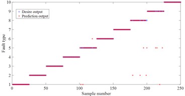
a) LSSVM based on HDE
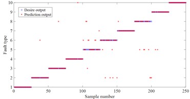
b) LSSVM based on MDE
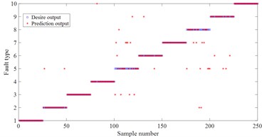
c) LSSVM based on MSE
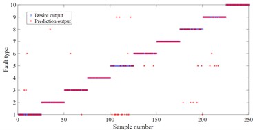
d) BP based on HDE
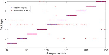
e) BP based on MDE
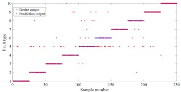
f) BP based on MSE
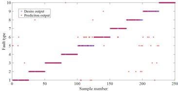
g) Bayes based on HDE
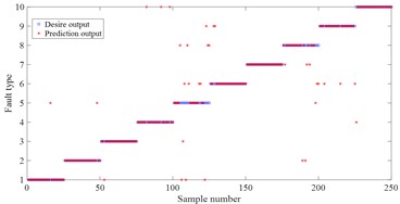
h) Bayes based on MDE
i) Bayes based on MSE
5. Conclusions
This paper proposes a rolling bearing fault diagnosis method based on the HDE and LSSVM. The effectiveness and practicability of the proposed method are verified by the vibration signals of the rolling bearing. The following conclusions are drawn as:
1) The proposed HDE based on LSSVM can be effectively applied in the fault diagnosis of rolling bearing.
2) HDE can consider the high-frequency and low-frequency components of rolling bearing. On this basis, HDE method can be effectively utilized to measure the complexity of rolling bearing and extract the effect feature vector for different fault types. Experiment results show that the proposed method has higher classification accuracy than the traditional method, MSE, and MDE.
3) Although with higher fault diagnosis accuracy, the new method still in the experimental verification stage based on the rolling bearing experiment system. In terms of this problem, the ability to resist noise should be further improved to make this method more effective in the actual working environment in the future.
References
-
Z. Chen and W. Li, “Multisensor feature fusion for bearing fault diagnosis using sparse autoencoder and deep belief network,” IEEE Transactions on Instrumentation and Measurement, Vol. 66, No. 7, pp. 1693–1702, 2017, https://doi.org/10.1109/tim.2017.2669947
-
J. Li, X. Yao, X. Wang, Q. Yu, and Y. Zhang, “Multiscale local features learning based on BP neural network for rolling bearing intelligent fault diagnosis,” Measurement, Vol. 153, No. 1, p. 107419, Mar. 2020, https://doi.org/10.1016/j.measurement.2019.107419
-
R. Yan and R. X. Gao, “Approximate entropy as a diagnostic tool for machine health monitoring,” Mechanical Systems and Signal Processing, Vol. 21, No. 2, pp. 824–839, Feb. 2007, https://doi.org/10.1016/j.ymssp.2006.02.009
-
J. S. Richman and J. R. Moorman, “Physiological time-series analysis using approximate entropy and sample entropy,” American Journal of Physiology-Heart and Circulatory Physiology, Vol. 278, No. 6, pp. H2039–H2049, Jun. 2000, https://doi.org/10.1152/ajpheart.2000.278.6.h2039
-
R. Yan, Y. Liu, and R. X. Gao, “Permutation entropy: A nonlinear statistical measure for status characterization of rotary machines,” Mechanical Systems and Signal Processing, Vol. 29, No. 1, pp. 474–484, May 2012, https://doi.org/10.1016/j.ymssp.2011.11.022
-
M. Costa, A. L. Goldberger, and C.-K. Peng, “Multiscale entropy analysis of biological signals,” Physical Review E, Vol. 71, No. 2, pp. 1–18, Feb. 2005, https://doi.org/10.1103/physreve.71.021906
-
J. Zheng, H. Pan, S. Yang, and J. Cheng, “Generalized composite multiscale permutation entropy and Laplacian score based rolling bearing fault diagnosis,” Mechanical Systems and Signal Processing, Vol. 99, No. 20, pp. 229–243, Jan. 2018, https://doi.org/10.1016/j.ymssp.2017.06.011
-
W. Yang, P. Zhang, and H. Wang, “Gear fault diagnosis based on EEMD multi-scale fuzzy entropy,” Journal of Vibration and Shock, Vol. 34, No. 14, pp. 163–167, 2015, https://doi.org/10.13465/j.cnki.jvs.2015.14.028
-
Y. Jiang, C.-K. Peng, and Y. Xu, “Hierarchical entropy analysis for biological signals,” Journal of Computational and Applied Mathematics, Vol. 236, No. 5, pp. 728–742, Oct. 2011, https://doi.org/10.1016/j.cam.2011.06.007
-
Y. Li, M. Xu, H. Zhao, and W. Huang, “A study on rolling bearing fault diagnosis method based on hierarchical fuzzy entropy and ISVM-BT,” Journal of Vibration Engineering, Vol. 29, No. 1, pp. 184–192, 2016, https://doi.org/10.16385/j.cnki.issn.1004-4523.2016.01.023
-
M. Rostaghi and H. Azami, “Dispersion entropy: a measure for time-series analysis,” IEEE Signal Processing Letters, Vol. 23, No. 5, pp. 610–614, 2016, https://doi.org/10.1109/lsp
-
H. Azami et al., “Multiscale Fluctuation-based dispersion entropy and its applications to neurological diseases,” IEEE Access, Vol. 7, No. 1, pp. 68718–68733, 2019, https://doi.org/10.1109/access.2019.2918560
-
P. Yao, K. Zhou, and Q. Zhu, “Quantitative evaluation method of arc sound spectrum based on sample entropy,” Mechanical Systems and Signal Processing, Vol. 92, No. 1, pp. 379–390, Aug. 2017, https://doi.org/10.1016/j.ymssp.2017.01.016
-
L. Si, Z. Wang, and X. Liu, “A sensing identification method for shearer cutting state based on modified multi-scale fuzzy entropy and support vector machine,” Engineering Applications of Artificial Intelligence, Vol. 78, No. 1, pp. 86–101, 2018, https://doi.org/10.1016/j.engappai
-
J. Zheng, Z. Dong, H. Pan, Q. Ni, T. Liu, and J. Zhang, “Composite multi-scale weighted permutation entropy and extreme learning machine based intelligent fault diagnosis for rolling bearing,” Measurement, Vol. 143, No. 1, pp. 69–80, Sep. 2019, https://doi.org/10.1016/j.measurement.2019.05.002
-
J. Suykens and A. Johan, “Least squares support vector machines,” International Journal of Circuit Theory and Applications, Vol. 2, No. 1, pp. 1–27, 2002.
Cited by
About this article

Public Projects of Zhejiang Province (LGF18F030003) and sponsored by K. C. Wong Magna Fund in Ningbo University.
