Bearing fault diagnosis using a novel coding-statistic feature combined with NNC

1. Introduction

Rolling bearings, as the extremely essential support components in rotating machinery, are most widely used in industrial machines. Their failures may generally result in machine breakdowns, and even casualties [1]. Hence, it is essential to diagnose their faults accurately and rapidly, especially for industrial site.

In general, three procedures are commonly included in bearing fault diagnosis. The first is to collect monitoring data with sensors. The second is to process the acquired signals to extract sensitive features related to the bearing health state. And the third is to diagnose bearing health conditions and/or locate the corresponding faults. The aforementioned fault features are usually extracted from raw signals in time domain, frequency domain and time-frequency domain. Time domain analysis is directly analyzed base on the time waveform of the vibration signals to extract features such as root-mean-square amplitude, skewness, kurtosis etc. [2]. Frequency domain analysis is often conducted with transforming vibration signals into frequency domain via fast Fourier transform to extract features such as cepstrum, Hilbert envelope spectrum analysis etc. [3], [4]. Time-frequency features are usually abstracted by means of short time Fourier transform [5], empirical mode decomposition [6], Wigner-Ville distribution [7], wavelet analysis [8], HHT time-frequency analysis, and high order spectral analysis [9]. However, the efficiency of the extraction process is of great importance for real-time diagnosis. Hence, more attentions should be focused on the phase of feature extraction for fault diagnosis.

Once the characteristics are extracted, bearing health state can be identified with assistance from one or more classifiers, such as distance classifiers, artificial neural networks (ANNs), support vector machines (SVMs) and so on. For example, Liu et al. [10] performed bearing fault diagnosis with LS-SVM and Empirical Mode Decomposition. Yang et al [11] conducted fault diagnosis of rolling bearing based on SVMs and fractal dimension. Sreejith et al. [12] employed time-domain features and neural networks for bearing fault diagnosis. And deep learning algorithm are utilized for fault diagnosis of rotating machine for the past few years [13], [14]. In general, artificial intelligence (AI) approaches, like ANNs and SVMs, may show an improved performance over other approaches. But in practice, however, it’s not easy to apply AI techniques to provide effective decision support due to their expensive computations. Considered their shortcomings, a simple classifier, nearest neighbor classifier (NNC), is employed in this study to classify the health states of bearings.

In this paper, a novel feature extraction method is proposed based on a coding strategy. First, a waveform coding matrix (WCM) is drawn from the time discrete series using a coding technique to capture the signal structures, and a coding-statistic feature is acquired from WCM with a pre-defined dictionary. Then two-dimensional principal component analysis (2DPCA) is employed to process these statistical features so that the redundancy and dimensionality of raw features could be rejected and reduced. Finally, an NNC is applied to classify the bearing faults. The main contributions of this work are to propose a new feature derived directly from time domain signal to interpret the health state of rolling bearings, and to perform fault diagnosis with 2DPCA and NNC.

The remainder of this paper is organized as follows. Section 2 presents the process of feature extraction using a coding strategy and statistical analysis in detail. Section 3 is dedicated to elaborating the proposed fault diagnosis scheme. And Section 4 provides the experimental validation with simulation and real data. Then lastly, the conclusions are presented in Section 5 together with possible future work.

2. Coding-statistic feature extraction

In this paper, a numeric coding technique is introduced to draw the information structures of collected signals at the feature extraction procedure. Suppose that the discrete time signal is $x=[x_1,x_2,\cdots ,x_{L-1},x_L]$, where $L$ represents the length of $x$, then the process of the proposed feature extraction can be summarized as follows.

Step 1: Perform zero-mean and normalization processing. In order to eliminate the influence of the mean and to meet the requirements of discrete coding, the discrete time series are first centered to have mean 0 and scaled to have standard deviation 1 according to standardized $z$-scores algorithm, and then normalized with min-max normalization method as described in Eq. (1):

where $i=\mathrm{1,2},\cdots ,L$, and $max\left(x\right)$, $min\left(x\right)$ denote the maximum and minimum of $x$ respectively. In particular, the maximum and minimum, i.e. $max\left(x\right)$ and $min\left(x\right)$, should be calculated through current encoded signals when applying online monitoring system. That is, they are computed from the new series which are obtained by splicing the repetitive points what acquired last time with the new collected discrete ones. In practice, they can be specified manually and empirically. Finally, the discrete time series are normalized as values between –1 and 1.

Step 2: Encode $x_{norm}$ as integers using $2^n$-level quantization. Uniform quantization considers the number range of equal divisions for creating region segments. In order to capture the structure of the time-domain waveform, uniform quantization is employed in this study, and the corresponding function “uencode” available in Matlab software has been used for this purpose. The syntax for this function is presented as “$y=$ uencode ($u$, $n$)”, where u is the normalized series in previous step and $n$ denotes the number of levels for quantization and n must be an integer between 2 and 32 (inclusive). In general, the value of n is recommended to specify between 7 and 12. The quantization rules are:

(1) If the input $u$ is less than –1, the value of the output of “uencode” is 0.

(2) If the input $u$ is greater than 1, the value of the output of “uencode” is $2^n-1$.

(3) The elements of the output y are unsigned integers with magnitudes in the range [0, $2^n-1$].

Finally, $x_{norm}$ can be encoded to integer values by applying $2^n$-level quantization as follows:

where adding “1” is to ensure the minimum element of $Y$ is one so as to generate the WCM in next step.

Step 3: Calculate the waveform coding matrix (WCM). Since the result of uniform quantization is obtained in step 2, the WCM can be constructed as $F\in R^{2^n\times L}$ by labeling its elements with “0” or “1”. The labeling rule is: label the element of $F$ as “1” at the location of the quantization output of $x_{norm}\left(i\right)$; otherwise, label the element of $F$ as “0”.

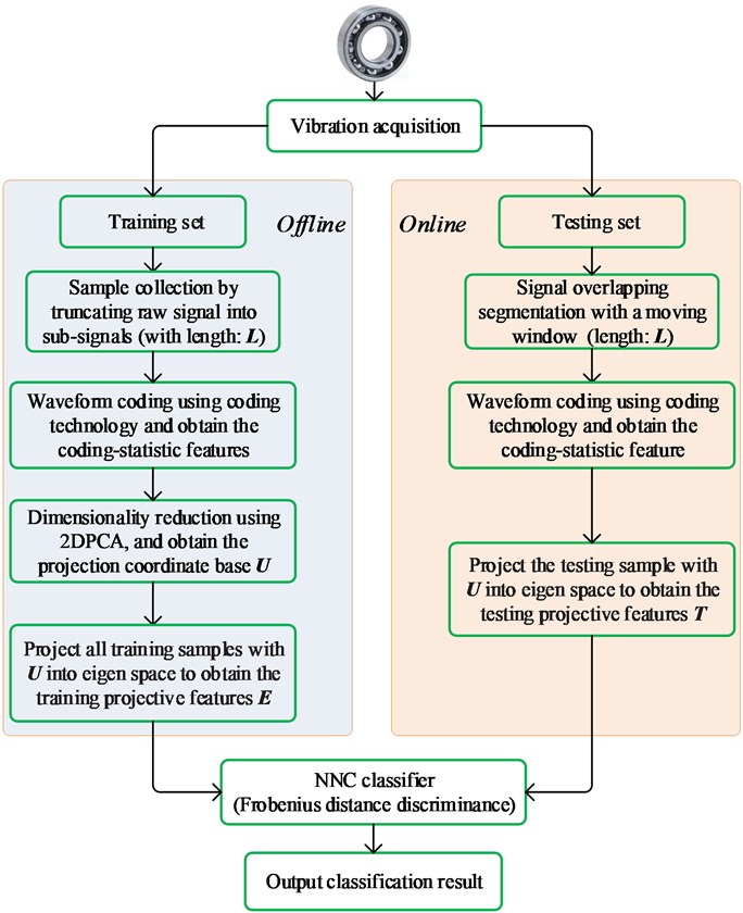
Fig. 1Technological process of the proposed feature extraction

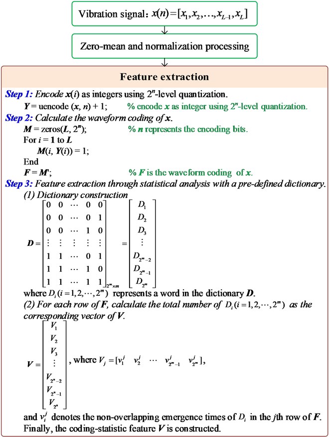
Step 4: Feature extraction through statistical analysis with a pre-defined dictionary. In order to perform feature extraction with the WCM of $x$, a dictionary $\mathit{D}$ is predefined as Eq. (3) at the very start:

where $D_i\mathrm{}(i=\mathrm{1,2},\cdots ,2^m)$ stands for a word in dictionary $\mathbf{D}$ with length $m$. Afterward, the total number of each word $D_i$ in every row of $\mathbf{F}$ is calculated, and then arranged in a statistical matrix $V_j\mathrm{}(j=\mathrm{1,2},\cdots ,2^n)$, each element of which denotes the non-overlapping emergence times of $D_i$. A coding-statistic feature $\mathbf{V}$ is constructed through the statistical analysis of $\mathbf{F}$ with the pre-defined dictionary $\mathbf{D}$ in the end.

The detailed step descriptions are presented in Fig. 1. As illustrated in Fig. 1, the calculation efficiency of the proposed coding form can be highlighted due to its omitting for the repetitive segments, especially for real-time condition monitoring system.

Next, the online computing process of the WCM is depicted with a simple parameter setting and the statistical feature extraction is illustrated intuitively. Fig. 2 gives an example of real-time waveform coding in condition monitoring system. Here, the sample length is set to $L=$ 18, and the quantization parameter is set to $n=$ 4.

Fig. 2An example of online waveform coding in condition monitoring system

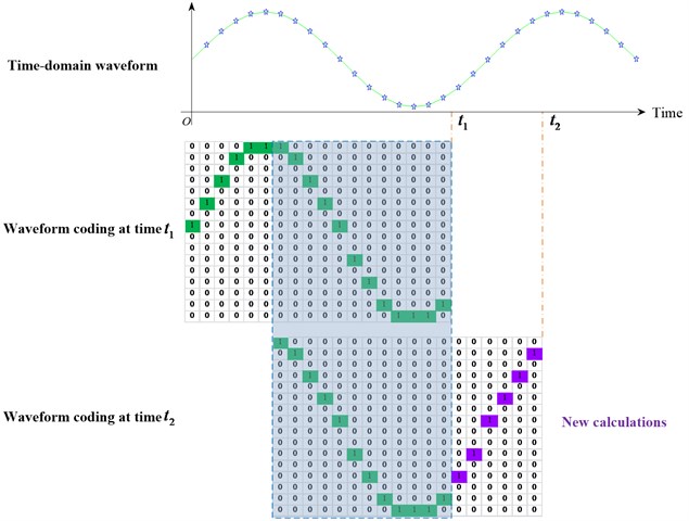
In the beginning, the waveform coding of signal acquired at time $t_1$ is performed to obtain the first WCM. While collecting the second coding sample at time $t_2$, these parts marked with grey box, which belong to repetitive calculations, cannot be encoded to reduce computational burden. Hence, only those parts whose elements are marked as pink, are calculated via waveform coding algorithm. Eventually the second waveform coding is obtained by combining the repeated coding ones with the new coding ones. From the computing process, it can be seen that the computation complexity is reduced thanks to this manipulation.

In the stage of statistical feature extraction, for simplicity, the length of word in pre-defined dictionary is set to $m=$ 3. Then the dictionary $\mathbf{D}$ is determined as follows:

where $D_1$ – $D_8$ denote the words in dictionary $\mathbf{D}$.

To illustrate the generating process of the statistical feature intuitively, the feature extraction process is presented in detail using the WCM at time $t_1$ shown in Fig. 2. The WCM at time $t_1$ is denoted as follows:

For example, the calculating process of the first row of $\mathbf{F}$ in Eq. (5) can be denoted as:

Then the feature extraction can be performed with the dictionary defined in Eq. (4). The calculating process of the feature for $F_1$ is illustrated in Fig. 3.

Fig. 3The feature extracting process of the 1st row of F (i.e. F1)

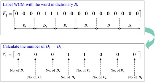
Finally, with the words $D_1$ – $D_8$ in dictionary $\mathbf{D}$, statistical feature $\mathbf{V}$ at time $t_1$ can be obtained using counting for certain word occurrence on each row of $\mathbf{F}$ presented in Eq. (5). The calculated feature $\mathbf{V}$ is shown in Eq. (7).

From the calculation process of feature extraction, it can be emphasized that the length of the sliding window ($L$) can be assigned to a larger size to contain more structure information about the analyzed object in real applications. Nevertheless, a high computational efficiency will be still retained for condition monitoring:

In subsequent section, the fault diagnosis scheme using the derived statistical features will be presented combined with 2DPCA and NNC.

3. The proposed fault diagnosis scheme

3.3. The proposed scheme for bearing diagnosis

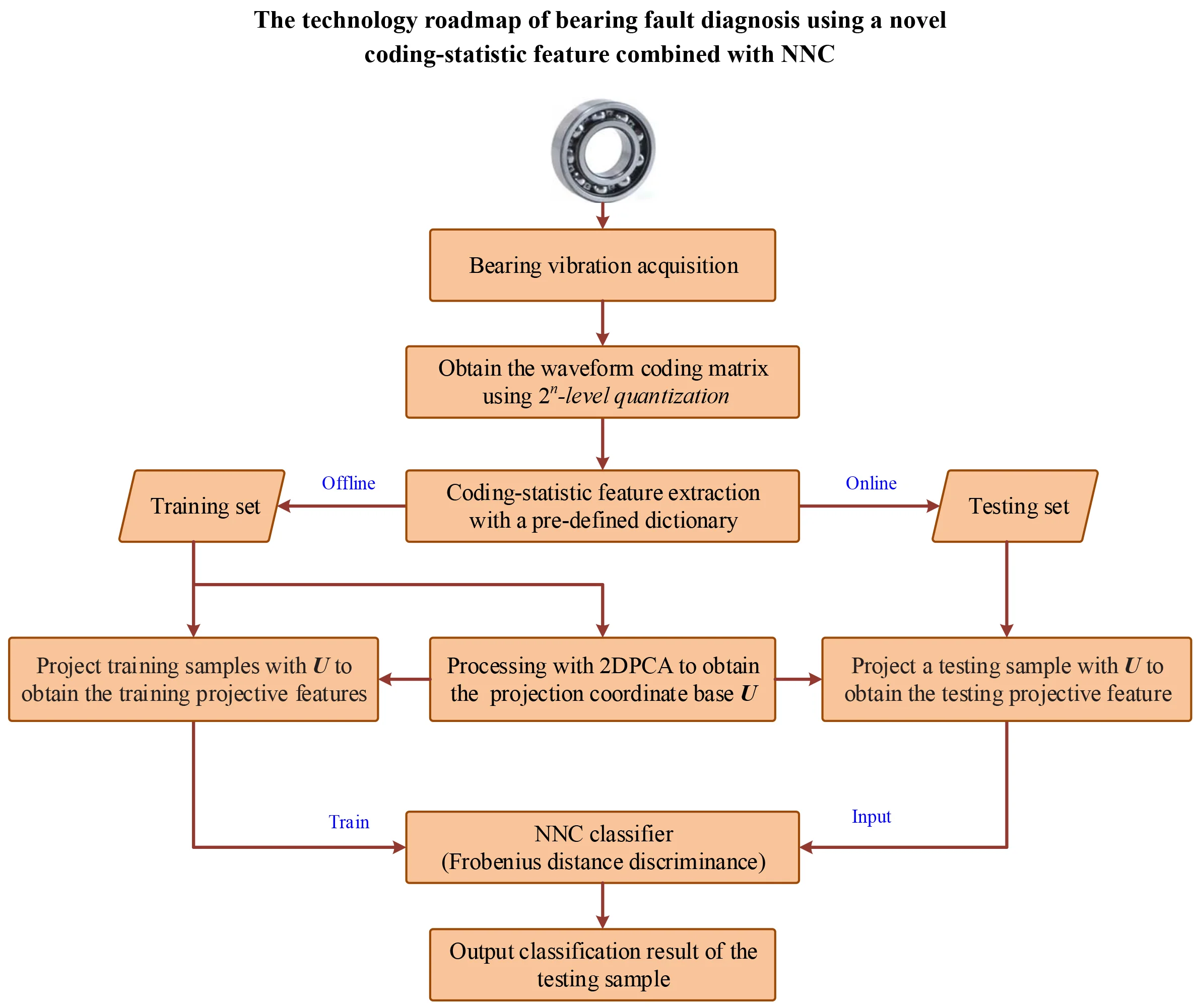
The framework of the proposed scheme for bearing diagnosis is depicted in Fig. 4.

The proposed method is decomposed into two main steps. The first step is done offline and aims at generating a classification model. The second step, which is achieved online, utilizes the model generated in the first step to classify the bearing health state. The process of the proposed method for offline training is given below:

(1) Vibration signal is first measured from the bearing system using acceleration sensors.

(2) Divide the original signal into equal time segments with a sliding window (length: $L$) and M sub-signals are obtained.

(3) Perform feature extraction according to the methodology described in section 2.

(4) Reduce dimensionality and remove redundancy using 2DPCA, and obtain the projection coordinate $U$.

(5) Train NNC model by projecting all training samples with $\mathbf{U}$ into eigen space to obtain the training projective features $E_j$ ($j=$1, 2,…, $M$).

For online fault diagnosis, the testing vibration signal is also acquired with length $L$, and the same process of WCM-based feature extraction is conducted to derive the original feature. Finally, it is input into the NNC model to decide its current state. In addition, the computation complexity of the proposed method could be less than the traditional fault diagnosis methods, due to the WCM is derived by a slipping scheme in feature extraction phase when applied in online monitoring.

Fig. 4Framework of the proposed diagnostic scheme

4. Experimental validation

4.1. Simulation study

To express the structures of the collected signals using the proposed coding technology more intuitively, a simulation presentation was conducted first. In this subsection, an impulse signal is employed to observe the performance of the waveform coding. An modified impulse signal from Ref. [17] is expressed in Eq. (17):

17

$y\left(k\right)=\sum _k{e}^{-900\times \left(k-r\times \frac{F_s}{f_m}-{\tau }_r\right)}+\mathrm{s}\mathrm{i}\mathrm{n}\left(2\pi f\times \frac{k-r\times \frac{F_s}{f_m}-{\tau }_r}{F_s}\right),$

where $f_m$, $f$ are equal to 110 and 3,900 respectively, the uniformly distributed random number $\tau \in [-0.1,\mathrm{}0.1]$ is used to simulate the randomness caused by the slippage, $F_s$ is the sampling frequency ($F_s=$ 12,000 Hz). And $(k-r\times F_s/f_m-{\tau }_r)/F_s)\ge 0$ is applied to ensure the causality of the exponential function.

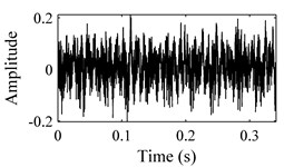
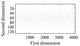
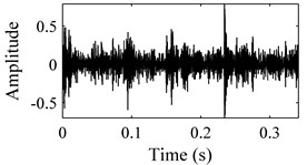
Fig. 5Impulse signal: a) time waveform; b) WCM of a)

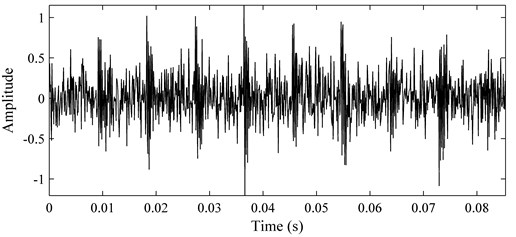
a)

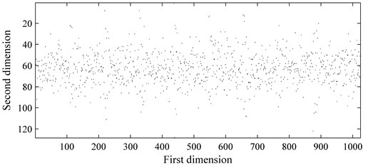
b)

In this chapter, the presence of additive Gaussian noise for the simulated signals are considered, and the signal noise ratio (SNR) is set as –2 dB. This simulation study aims to show the waveform coding process of the proposed method. According to the generation process of WCM, it can be seen that the WCM can be dug as the eigenstate of the simulated signals. It is clear that, the intrinsic structure of the analyzed signal is exploited into a two-dimensional matrix. The original signal and its WCM are shown in Fig. 5, where only 1024 sampling points are displayed.

The feature extraction of the simulated data is omitted on account of the large length of the signals (i.e., $L=$ 1024), with which the feature matrix $\mathbf{V}$ is too large to demonstrate here. For the technical details about feature extraction, readers can refer to the example presented in Fig. 3.

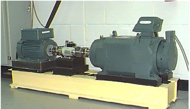
Fig. 6The test rig for bearing fault diagnosis

4.2. Bearing fault diagnosis using the proposed method

4.2.1. Bearing data description

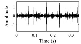
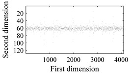
In order to evaluate the performance of the proposed methodology, vibration signals collected from Case Western Reserve University [18] are utilized to validate the effectiveness of the diagnostic scheme. As depicted in Fig. 6, the test rig consists of a 2 hp motor (left), a torque transducer/encoder (center), a dynamometer (right), and control electronics (not shown). Bearing with fault diameters of 0.007 inches, 0.014 inches, 0.021 inches, 0.028 inches, were installed on the motor housing at the drive end of the motor to acquire the vibration signals. Vibration signals under four different load/speed conditions, i.e. C1 = 0 hp/1797 rpm, C2 = 1 hp/1772 rpm, C3 = 2 hp/1750 rpm and C4 = 3 hp/1730 rpm, were collected with a sampling frequency of 1,2000 Hz. The experiment conditions are illustrated in Table 1. The bearing data sets were obtained from the experimental bench under the four different health conditions: (1) normal condition (NO); (2) with inner race fault (IF); (3) with outer race fault (OF); and (4) with ball fault (BF). Fig. 7 illustrates the WCMs obtained from bearings under different health status in C3 operating condition. In this work, the length of the sub-signal (or the moving window) is set as 4096, and the quantization bit n and word length m are empirically designated as 7 and 3 respectively.

Fig. 7Time-domain waveforms and WCMs of four different operation statuses in C3 condition: a), b) normal condition; c), d) inner race fault; e), f) ball fault and g), h) outer race fault

a)

b)

c)

d)

e)

f)

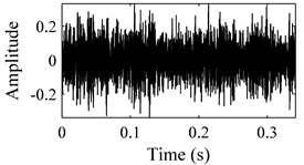
g)

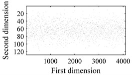
g)

Table 1Illustration of the experiment conditions

Experiment conditions	C1	C2	C3	C4
Speed (rpm)	1797	1772	1750	1730
Load (hp)	0	1	2	3

In this section, two experiments were conducted over two different data subsets (A-B) to fully verify the robustness of the proposed method. During the random segmentation phase, the samples were randomly extracted with a fix time window from the acquired raw vibration signals. And 200 samples were created for each bearing with NO (or IF, or OF and or BF) under load condition C1 (or C2, or C3 and or C4). The two classification problems are summarized in Table 2.

Table 2Description of the bearing data sets

Data set	No. of samples (training/testing)	Defect size (training/testing)	Health condition	Label
A	400/400	0/0	Normal	1A
	400/400	0.007/0.007	Ball fault	2A
	400/400	0.007/0.007	Inner race fault	3A
	400/400	0.007/0.007	Outer race fault	4A
B	400/400	0/0	Normal	1B
	400/400	0.007/0.007	Ball fault	2B
	400/400	0.014/0.014	Ball fault	3B
	400/400	0.021/0.021	Ball fault	4B
	400/400	0.007/0.007	Inner race fault	5B
	400/400	0.014/0.014	Inner race fault	6B
	400/400	0.021/0.021	Inner race fault	7B
	400/400	0.007/0.007	Outer race fault	8B
	400/400	0.014/0.014	Outer race fault	9B
	400/400	0.021/0.021	Outer race fault	10B

Table 3Diagnosis performance using the proposed method

Data set	Testing condition				Average accuracy
	C1 (0 hp/1797 rpm)	C2 (1 hp/1772 rpm)	C3 (2 hp/1750 rpm)	C4 (3 hp/1730 rpm)
A	94.30 %	95.36 %	95.15 %	91.88 %	94.42 %
B	95.65 %	95.47 %	95.06 %	93.07 %	94.81 %

4.2.2. Diagnostic performance analysis

In order to eliminate the redundancy of the original coding statistic features and improve the computational efficiency, all collected original features for training sets are tackled by means of 2DPCA algorithm to calculate the projection coordinate for reduction of dimensionality. While processing using 2DPCA, the contribution of the selected largest eigenvalues is set as $\gamma =$ 90 %, to establish the projection coordinate. Then the original training and testing features are mapped with the projection basis. As a result, the NNC is trained with the dimension-reduced features of training samples to derive the state classification model. One other thing to note is that training samples under the four load conditions are all applied to train the NNC model in the training phase, and each experimental routine is performed 20 times via randomly selecting training samples, then the average accuracies of the 20 randomized trials are calculated and recorded. The diagnostic performances of the two data sets are shown in Table 3.

Examining the diagnostic performance from Table 3, it can be observed that high accuracies are achieved for both data set A and B. For the first classification problem, testing samples from C1, C2, C3 and C4 were classified with accuracy 94.30 %, 95.36 %, 95.15 % and 91.88 % respectively. Average accuracy, 94.42 %, is obtained and it indicates that the proposed method could diagnose the health states of bearing with satisfied performance. Moreover, for the second classification problem, testing samples from C1, C2, C3 and C4 were classified with accuracy 95.65 %, 95.47 %, 95.06 % and 93.07 % respectively. This shows that the proposed method could be capable of handling this multi-class problem to perform bearing fault classification. Meanwhile, an interesting phenomenon is noticed that the average accuracy using data set B (10 class) is little higher than that using data set A (4 class). The main reason is that the samples in the class of 2B, 5B and 8B are more misclassified than others.

In order to compare the performance for fault diagnosis more intuitively, some published publications are convened to make comparisons in Table 4.

Table 4Diagnostic performance comparison with some published works

Method	Load condition	Classified problem (training/testing)	Accuracy (%)
Multiple ANFIS combination [19]	Multiple	4 class (both 0.007)	100.00
		10 class (both 0, 0.007, 0.014, 0.021)	91.33
SVR + phase space features [20]	Single	10 class (both 0, 0.007, 0.014, 0.021)	90.30
TR-LDA2 + kNN classifier [21]	Single	10 class (both 0, 0.007, 0.014, 0.021)	92.50-98.00
NNC + coding features [present work]	Multiple	4 class (both 0.007)	94.42
		10 class (both 0, 0.007, 0.014, 0.021)	94.81

Validating with the same bearing data, time- and frequency-domain features are calculated and classified with multiple adaptive neuro-fuzzy inference system (ANFIS) combination in [19], in which 100.00 % and 91.33 % are obtained for the two classification problems respectively. As for the ten-class classification problem, phase space features and Support Vector Regression Machine (SVR) in [20], trace ratio criterion LDA (TR-LDA) and kNN classifier in [21] are put forward to deal with this complicated situation, and accuracies of 90.30 %, 92.50-98.00 % and 99.38 % are obtained respectively. Meanwhile, the present work with 94.81 % classification accuracy seems to be another excellent diagnostic method in handling this problem. Through the comparison and analysis, it can be seen that the proposed diagnostic scheme could demonstrate excellent performance on fault classification problems, overall. Due to the excellent efficiency of feature extraction and the outstanding performance for fault classification, the proposed method is also applicable to be applied in the fault diagnosis system for industrial applications.

5. Conclusions

Obviously, the waveform coding algorithm proves that the nature and regularity of the time series could be grasped deeply. More and higher requirements are being put forward for industrial applications, as well as the efficiency of the utilized algorithms is receiving more and more attentions. Based on this consideration, a WCM-based feature extraction method is proposed in this paper. At first, the statistical feature is acquired directly from WCM of the time domain series with the assistance of a coding algorithm. Then 2DPCA is employed to tackle these statistical features obtained in previous phase. Finally, fault classification with NNC is applied for classification. Two groups of experiments are conducted to validate the performance of the presented methodology. Reviewing the process of feature extraction and the effectiveness for fault classification, some conclusions are derived as follows.

1) The proposed algorithm has small algorithmic complexity and high efficiency. Thanks to its non-repetitive calculation for the overlapping sections as illustrated in Fig. 2, the proposed algorithm is well suited for online monitoring in real-time fault diagnosis systems.

2) The diagnosis scheme in this paper could show an excellent performance in handling the multi-class classification problems like data set B in Table 2.

As described in Section 2, it can be seen that the parameter $n$ for quantization and $m$ for WCM-based feature calculation may influence the performance and robustness of the proposed coding method. And they are both selected empirically. Therefore, a future work will be aimed at the optimized selection of these parameters to further improve the robustness of the proposed method.