Abstract
This paper firstly introduced the theory and implementation of the least squares complex frequency domain (LSCF) method based on the truncated singular value decomposition (SVD) for noise reduction. The simulation results of signals with different signal noise ratios (SNR) show that this algorithm is stable and has excellent capacity of resisting noise disturbance. On this basis, an online detection system for natural frequency of brake discs is developed. This system takes the LAN-XI date acquisition module and LABSHOP software of B&K as platform and uses Visual Basic (VB) and MATLAB mixed programming technique for its secondary development. The LSCF method based on the truncated SVD is applied for curve fitting and modal parameter extracting. The qualified criterion is that the stably appearing natural frequencies are in the tolerance ranges. The practical application shows that this system intuitively and accurately displays the detection results and performs stably and efficiently.
1. Introduction
Online detection technique based on the identification of natural frequency has been an important method for the quality evaluation of brake discs. Companies, like Ford, TRW, etc. employ online detection system to ensure their brake discs’ quality. They judge whether the product is qualified by detecting whether the low order natural frequencies are in the tolerance ranges [1, 2]. The pick picking (PP) method was once applied to online detection system as the identification method for natural frequency and unqualified products were kicked out in some degree [2]. However, the PP method is an image processing way that has a high-quality requirement in the measured frequency response function, which limits the stability of online detection. The well-known least squares complex exponential (LSCE) method [3] is an effective curve fitting way in time-domain, but is easily affected by large noise in the factory and not applied to online detection widely. In recent years, El-Kafafy et al. [4, 5] presented a modal parameter identification method called maximum likelihood modal model-based (ML-MM) which improved the quality of the modal model in terms of the bias and variance for the modal parameters compared to the existing well-known LSCF method. But it costs much time in iteration operation and will decrease the efficiency of online detection. In fact, LSCF method is a widely-used frequency-domain modal parameter estimation method, and it has higher accuracy and stability than the PP and LSCE method and also a faster calculation speed than the existing iterative method [5-8].
The above algorithms estimate the parameters from the measured frequency response function directly without noise reduction for the signal, when applied to online detection system, the accuracy is not assured for the large noise in the production line. So, an appropriate noise reduction method is needed. Inspired by the most recent methods of component damage detection [9, 10], an improved LSCF method is presented, which combines LSCF method for modal parameter identification and SVD algorithm for noise reduction and is applied to online detection system for natural frequency of brake discs. The system takes the LAN-XI date acquisition module and LABSHOP software of B&K as platform and uses Visual Basic (VB) and MATLAB mixed programming technique for its secondary development.
2. Algorithm implementation
In the developed system, the improved LSCF method is programmed by MATLAB, and the measured data are processed by the truncated SVD algorithm for noise reduction, and modal parameters are extracted automatically based on the clarified stabilization diagram technique [11]. These developed algorithms make the system run automatically and the identification result accurate and consistent.
2.1. The LSCF method
The LSCF method is based on the common denominator model of the frequency response function [12, 13]. The coefficients of the denominator polynomial are solved by minimizing the error between model and measured data, and then the poles are solved from the eigenvalue of the companion matrix of the polynomial with the solved coefficients. The natural frequency and damping ratio are further solved from the poles.
The common denominator model of frequency response function is:
With the frequency response function, ( the serial number, the -th frequency, and the coefficients of numerator and denominator polynomial respectively, the polynomial basis function and the polynomial order ( the model order of the frequency response function). , where is the frequency resolution. In the LSCF method, a discrete time domain model [11] is applied and let be the discrete time interval, which can be formulated as:
And can be formulated as:
Replace with the measured frequency response function and construct the error function based on Eq. (1) as:
To minimize the value of error function, the least square equation is formulated as:
with and:
To speed up the solving speed of Eq. (5), left multiply it by and reformulate the normal equation as:
With the real part component of a complex, and The coefficients of numerator polynomial can be expressed by from the first row of Eq. (11) as:
Substitute into the second row of Eq. (11) and get the reduced normal equation as:
To solve the coefficients of denominator polynomial and get a clarified stabilization diagram, a constraint must be applied to . Cauberghe et al. [14] studied the relationship between the constraints and poles and pointed out that the constraint equation results in the damping ratio of mathematic poles negative. The physical poles can be effectively selected from mathematic poles based on this. So, the coefficients of denominator polynomial can be solved by substituting into Eq. (13).
With determined, Eq. (14) corresponding to the denominator polynomial can be solved:
And the poles are solved from the roots of Eq. (14). However, when the model order is too high, it is difficult to solve the equation directly. The problem about solving the poles of the frequency response function can be transformed into solving the eigenvalue of the companion matrix of the polynomial with coefficients . Decompose matrix by the eigenvalue as:
With the eigenvector matrix, the diagonal matrix with eigenvalues. The roots of Eq. (14) are in the diagonal line of eigenvalue matrix , and , where is the -th eigenvalue and is the corresponding pole. The natural frequency and damping ratio can be solved from the real and imaginary parts of .
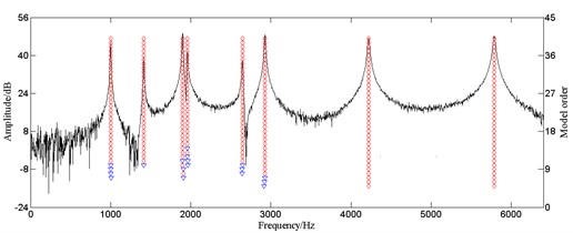
A certain type of brake disc is detected to extract the frequency response function as an example. The stabilization diagram by the LSCF method is shown as Fig. 1.
Fig. 1Stabilization diagram of the LSCF method (◇: both frequency and damping ratio stable; ▽: only frequency stable)
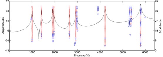
The red diamond indicates poles that are stable in both frequency and damping ratio, and the inverse blue triangle indicates poles only stable in frequency. The stability of poles is determined by the change rate of frequency and damping ratio of adjacent model order. If both of them are in the tolerance ranges, the pole is seen as stable pole. If only the frequency change ratio is in the tolerance range, the pole is seen as only frequency stable pole. If the occurrence number of both frequency and damping ratio stable pole, that’s the number of red diamond in a certain column of the stabilization diagram, is one-third greater than the maximum model order, the corresponding frequency is seen as natural frequency, or the poles are seen as only frequency stable poles. The occurrence of only frequency stable poles is very likely to cause error in natural frequency extraction.
The identification result is credible for the poles steadily appear in the peaks of the frequency response function curve as shown in Fig. 1. However, there are many only frequency stable poles at about 2960 Hz, 3898 Hz, 5276 Hz, and 5372 Hz, which appear as small peaks. Small peaks are sensitive to the small change of excitation positions and SNR, so they are not acceptable to be the criteria of online detection. Besides, noise interference does harm to the accuracy of online detection. So, it is necessary to apply the truncated SVD algorithm to the LSCF method for noise reduction, thus increasing its accuracy and anti-noise interference ability.
2.2. Truncated SVD for noise reduction
In signal processing, SVD has been proved to be an effective method for noise reduction by restraining small signal components to enhance large components [15]. Considering that the SVD is completed in the time domain, the frequency response function is firstly transformed to impulse response function. And after the noise reduction is done, the processed signal is transformed back into the frequency domain for modal parameter identification by the LSCF method.
Based on the theory of phase space reconstruction [16], the transformed impulse response function can be seen as the original signal with noise interference. When it is mapped into a demission phase space, the reconstructed phase space orbit matrix is:
Obviously, is a Hankel matrix and .
Matrix indicates the evolution properties of reconstructed attractor in phase space and can be expressed as: , with and , the orbit matrices of signal and noise respectively. So, the noise reduction for initial signal becomes the finding of optimal approximation for , with known ahead. Decompose matrix by the singular value as:
With , demission unitary matrix, , demission unitary matrix, and , demission positive semi-definite matrix. The singular values of are in the diagonal of with large to small arrangement. Truncate the first larger singular values while the rest are set as 0, and matrix is got from the inverse process of SVD by the equation: , where is the truncated demission matrix. Then, matrix is the optimal approximation to orbit matrix with truncated order , and noise is reduced at some degree. The order to be truncated in SVD is determined by the increment of singular entropy [17]. The singular entropy of truncated signal can be expressed as:
With the increment in the -th order and can be calculated by:
With the -th larger singular value. When a wide-band noise interferes in the signal, the singular entropy grows with the model order and the growing speed slows down at a certain value, where the effective feature information is almost saturate and the following increase of the singular entropy comes from noise. So, the chosen order for truncation is located at the slowed down order. In other words, the truncation order is determined by the value of , thus reserving effective signal component and removing noise component.
Generally, matrix is no longer a Hankel matrix and to get the de-noised signal matrix , the back-diagonal values of are averaged as Eq. (20). To simplify the calculation, the demission matrix is lower right zero padded to a demission matrix :
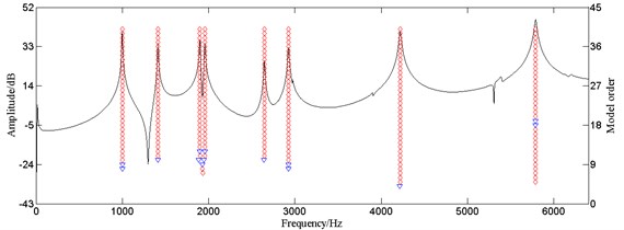
Fig. 2Stabilization diagram of the LSCF method with truncated SVD (◇: both frequency and damping ratio stable; ▽: only frequency stable)
Till then, transform the time domain signal back into the frequency domain as a new frequency response function and the modal parameters can be extracted by the LSCF method.
The frequency response function of brake disc from Fig. 1 is set as an example. The proposed algorithm, truncated SVD for noise reduction and the LSCF method for modal parameter identification, is applied to it. Stabilization diagram from that algorithm is shown as Fig. 2 and modal parameters are extracted in Table 1. It clearly shows that this algorithm effectively restrained small peaks and noise and the stabilization diagram is more clear and accurate than Fig. 1.
Table 1Identification results of the LSCF method with truncated SVD
Mode | Frequency / Hz | Damping / % |
1 | 999.6 | 0.28 |
2 | 1411.8 | 0.24 |
3 | 1897.7 | 0.22 |
4 | 1955.7 | 0.23 |
5 | 2644.5 | 0.19 |
6 | 2925.4 | 0.22 |
7 | 4219.8 | 0.27 |
8 | 5786.9 | 0.24 |
3. Validation of algorithm stability
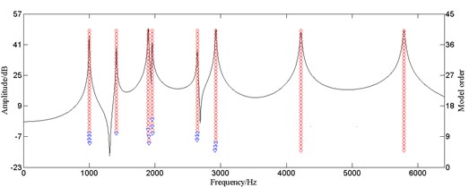
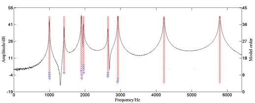
Online detection system works with unavoidable noise interference in signal transfer and collection, so the stability of the LSCF method based on truncated SVD should be validated. The frequency response function using the data in Table 1 is fitted and white Gaussian noises, respectively resulting in SNR of 50 dB, 30 dB, are added in it as calculation examples. The parameters are identified by the developed algorithm and the results are compared with the signal without noise. The stability diagrams are shown in Fig. 3.
The poles steadily appear in the stabilization diagram at the peaks of the response curve regardless of the SNR as shown in Fig. 3, indicating that the developed algorithm effectively restrained noise and the identification results are accurate. So, there is possibility for the application of this algorithm to online detection system for natural frequency of brake discs.
4. System development
Based on the previous proposed method, an online detection system for natural frequency of brake discs is developed. The hardware part is composed of 8206-002 force-hammer, 4507B4 acceleration sensor, 3050A LAN-XI data acquisition module of B&K and a personal computer. The software part is mainly the secondary development of VB and MATLAB based on PULSE LabShop, professional test software of B&K. In this system, key parameters are controlled in form of configuration file, so demands of different detection objects can be qualified easily, thus expanding the application range of this system.
4.1. Program development
The developed system is based on the mixed programming of VB and MATLAB. It mainly realizes the control and parameter settings of PULSE Lab Shop, the extraction of frequency response function, the identification of modal parameters, the qualified evaluation and data storage management. The frequency response function is extracted from PULSE Lab shop by VB and the LSCF method based on SVD developed by MATLAB is compiled by MATCOM into DLL file that can be called by VB. So, the parameter identification can be done in online detection process. The software flow chart is shown as Fig. 4.
Fig. 3Stabilization diagram of the LSCF method with truncated SVD under different SNR (◇: both frequency and damping ratio stable; ▽: only frequency stable)
a) Without noise
b) SNR = 50 dB
c) SNR = 30 dB
Fig. 4Flow chart of main program
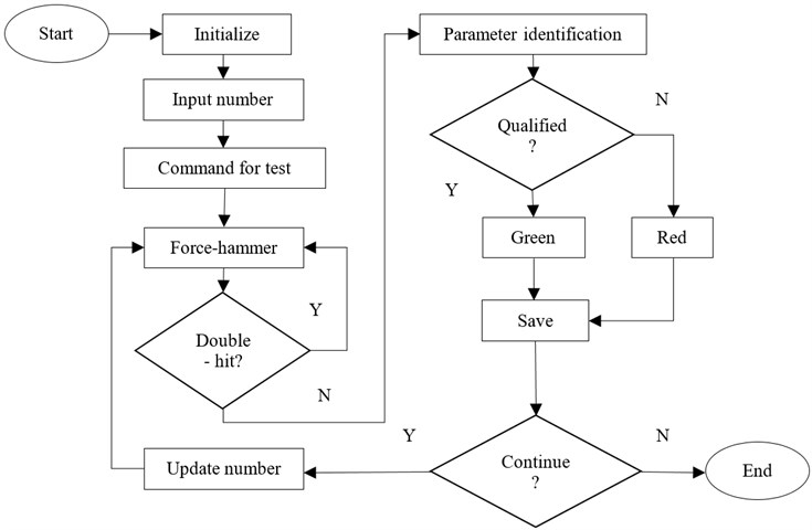
When the software works, PLUSE Lab Shop is firstly opened and the measurement parameters in the configuration file are read out and the system is initialized. This system saves all of the attribute parameters and testing numbers in form of configuration file, so the setting of constraint parameters and testing numbers are only necessary in the first detection of a new product. When clicking the start button, the software will send command to PULSE for detection and wait for excitation from force hammer. When the force signal and the corresponding acceleration signal are detected, the force signal is extracted for double hit detection. If double hit exists, the system will back to waiting for a new excitation from force-hammer, if not, the frequency response function will be extracted for modal parameter identification. Then, the extracted natural frequencies and reference natural frequencies are compared and qualification judgment is made. Finally, the qualified rate will be counted and saved automatically, and the frequency response function curve, double hit detection curve, natural frequencies and qualified result will be shown in the ‘Live Report’ that embedded in the main interface. The system has a continuously automatic detection principle that it updates the testing number and back to waiting for pulse excitation automatically, so the running efficiency is high. The main graphical user interface of this software is shown as Fig. 5.
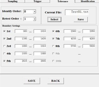
Small peaks in the frequency response function of brake discs are sensitive to the small change of excitation positions and if the corresponding frequencies are set as references, there might be misjudge. So, in this system, the frequencies that steadily appear and not easily affected by the small change of excitation positions are selected as references manually. If the corresponding natural frequencies are in the tolerance range, the product is judged as qualified. The Graphical user interface of tolerance settings is shown as Fig. 6.
Fig. 5Main graphical user interface of the software
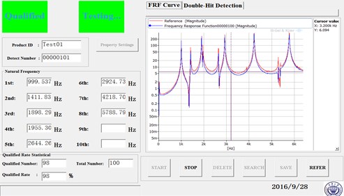
Fig. 6Graphical user interface of tolerance settings
4.2. Parametric control
For the convenience of adjusting constraint parameters according to different detection objects and user requirements, the key parameters are controlled in form of configuration file. This parametric control extends the application range of the system. The key parameters include the frequency range, the maximum model order and steady parameters.
The setting of frequency range not only defines the frequency width for parameter identification, but also constraints the data base that constructs the least square equations in LSCF algorithm. The sample capacity is required to be far more than two times the model order to avoid ill-conditioned functions.
The maximum model order is the maximum function order to be cyclically solved in LSCF algorithm. The model order should be as large as 30-50 to contain enough information of frequency response function and get more stable poles.
Steady parameters include the absolute and relative value of damping ratio tolerance and the relative value of frequency tolerance. The absolute value of damping ratio tolerance that usually at a small value is the upper limit of damping ratio. It is determined by the damping characteristic of the detected object. The relative value of frequency tolerance and damping ratio tolerance determine the stability of a pole, and the setting of the latter is often higher than the former for the frequency is easier to be stable because of its higher pure value. In this online detection system, the default setting tolerances of absolute and relative damping ratio and relative frequency are 10 %, 5 % and 1 % respectively.
5. Validation of system stability
In order to verify the stability of the developed system and set reference orders for its application to production line, the mentioned type of brake disc is detected for 100 times without the setting of reference orders and the statistic result is shown in Table 2. Because of the small change of excitation positions, some frequencies didn’t steadily appear. So, the frequencies that steadily appeared are selected as references and the tolerances are set at proper values for validation in real production line.
Table 2Frequency information of 100 detections
Mode | Minimum / Hz | Maximum / Hz | Appearance | Reference |
1 | 999.0 | 999.8 | 100 | √ |
2 | 1411.1 | 1412.3 | 100 | √ |
3 | 1897.1 | 1903.5 | 94 | × |
4 | 1954.0 | 1956.4 | 76 | × |
5 | 2642.6 | 2646.7 | 100 | √ |
6 | 2923.0 | 2931.5 | 100 | √ |
7 | 4217.7 | 4232.2 | 100 | √ |
8 | 5783.8 | 5792.8 | 91 | × |
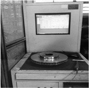
The developed system is applied to the production line of the mentioned brake disc and the photo of test field is shown as Fig. 7. The selected frequencies are the 1st, 2nd, 5th, 6th and 7th order frequencies from Table 2. The corresponding tolerance ranges are set and 900 brake discs produced in an eight-hour day are detected. A single detection takes about 30 s, with 18 s the installation of acceleration sensor and 12 s the working of the software, and the qualified rate is about 98.7 %. The application result shows that this system displays accurate result and operates stably with high efficiency.
Fig. 7Photo of engineering application in site
6. Conclusions
In this paper, an improved LSCF method is presented, which combines LSCF method for modal parameter identification and SVD algorithm for noise reduction and is applied to online detection system for natural frequency of brake discs. The simulation results show that the developed algorithm has excellent noise restraint ability and the identification result is reliable and shows good consistency.
The developed system has high efficiency for the application of continuous detection by updating the detection number automatically. The possibility of misjudgment from the small change of excitation positions is reduced by a combined judgment method. The application range is extended by the parametric control of key identification parameters. The application of this system to a certain brake disc production line shows that it has good performance of accuracy, stability and efficiency.
References
-
Chu Z. G., Ye F. B., Jiang Z. H., et al. Modal analysis of brake disc and its application to production-line inspection system. Automotive Engineering, Vol. 36, Issue 7, 2014, p. 843-847.
-
Chu Z. G., Wu Y. J., Xiong M., et al. Development of online detection system for natural frequency using impact test. Journal of Electronic Measurement and Instrument, Vol. 29, Issue 1, 2015, p. 31-37.
-
Brown D. L., Allemang R. J., Zimmerman R. D., et al. Parameter estimation techniques for modal analysis. SAE Paper, Vol. 88, Issue 2, 1979, p. 299-305.
-
El-Kafafy M., Troyer T. D., Guillaume P. Fast maximum-likelihood identification of modal parameters with uncertainty intervals: a modal model formulation with enhanced residual term. Mechanical Systems and Signal Processing, Vol. 48, 2014, p. 49–66.
-
El-Kafafy M., Peeters B., Guillaume P., et al. Constrained maximum likelihood modal parameter identification applied to structural dynamics. Mechanical Systems and Signal Processing, Vol. 72, Issue 73, 2016, p. 567-589.
-
Verboven P., Cauberghe B., Guillaume P. Improved total least squares estimators for modal analysis. Computers and Structures, Vol. 83, Issues 25-26, 2005, p. 2077-2085.
-
Alessandro F. Modal parameters estimation in the Z-domain. Mechanical Systems and Signal Processing, Vol. 23, Issue 1, 2009, p. 217-225.
-
Verboven P., Guillaume P., Cauberghe B., et al. Modal parameter estimation from input-output Fourier data using frequency-domain maximum likelihood identification. Journal of Sound and Vibration, Vol. 276, Issue 3-5, 2004, p. 957-979.
-
Zhang S. B., Lu S. L., He Q. B., et al. Time-varying singular value decomposition for periodic transient identification in bearing fault diagnosis. Journal of Sound and Vibration, Vol. 379, 2016, p. 213-231.
-
Kang M., Kim J-M. Singular value decomposition based feature extraction approaches for classifying faults of induction motors. Mechanical Systems and Signal Processing, Vol. 41, Issues 1-2, 2013, p. 348-356.
-
Van der Auweraer H., Guillaume P., Verboven P., et al. Application of a fast-stabilizing frequency domain parameter estimation method. Journal of Dynamic System, Measurement and Control, Vol. 123, Issue 4, 2001, p. 651-658.
-
Verboven P., Guillaume P., Cauberghe B., et, al. Frequency-domain generalized total least-squares identification for modal analysis. Journal of Sound and Vibration, Vol. 278, Issue 1-2, 2004, p. 21-38.
-
Verboven P. Frequency-Domain System Identification for Modal Analysis. Ph. D. Thesis, Department of Mechanical Engineering, Vrije Universiteit, Brussel, 2002.
-
Cauberghe B., Guillaume P., Verboven P., et al. The influence of the parameter constraint on the stability of the poles and the discrimination capabilities of the stabilisation diagrams. Mechanical Systems and Signal Processing, Vol. 19, Issue 5, 2005, p. 989-1040.
-
Braun S., Ram Y. M. Determination of structural modes via the Prony model: system order and noise induced poles. Journal of the Acoustical Society of America, Vol. 81, Issue 5, 1987, p. 1447-1459.
-
Lv Z. M., Zhang W. J., Xu J. W. A noise reduction method based singular spectrum and its application in machine fault diagnosis. Chinese Journal of Mechanical Engineering, Vol. 35, Issue 3, 1999, p. 85-88.
-
Yang W. X., Jiang J. S. Study on the singular entropy of mechanical signal. Chinese Journal of Mechanical Engineering, Vol. 36, Issue 12, 2000, p. 9-13.
About this article

This work was supported by grants from the National Natural Science Foundation of China (No. 51275538) and the Chongqing Significant Application and Development Planning Project (No. cstc2015yykfc60003).
