A study on Gabor frame for estimating instantaneous dynamic characteristics of structures

Su, Wei-Chih; Huang, Chiung-Shiann

doi:10.21595/jve.2016.17894

Journal of Vibroengineering

Browse Journal

Submit article

Published: 15 February 2017

Check for updates

A study on Gabor frame for estimating instantaneous dynamic characteristics of structures

Wei-Chih Su¹

Chiung-Shiann Huang²

¹National Center for High-Performance Computing, National Applied Research Laboratories, Hsinchu, 30076, Taiwan

²Department of Civil Engineering, National Chiao Tung University, Hsinchu, 30076, Taiwan

Corresponding Author:

Wei-Chih Su

Cite the article Download PDF

Downloads 1469

Abstract

A structure under damage normally exhibits nonlinear dynamic behaviors and time-dependent stiffness and damping. By estimating instantaneous dynamic characteristics of a structures is generally very useful when assessing structural damage in real application. This study presents a novel and effective approach that accurately estimating instantaneous dynamic characteristic of a structure using time-varying autoregressive exogenous (TVARX) model on Gabor frame. To evaluate the time-varying coefficient matrices of a time-series model, the proposed procedure applies Gaussian-based weighted function and Fourier transform on time series model, then the Gabor-transform-based time series formula could be obtained. The dynamic characteristics of a structure are determined from the coefficient matrices. Numerical analyses demonstrate that the proposed approach is superior to traditional time-frequency analysis in accurately estimating instantaneous dynamic characteristics of a structure. Finally, the proposed approach is applied to process measured data for a steel frame specimen subjected to a series of base excitations in shaking table tests.

1. Introduction

When a structure either subjected to severe loading like a strong earthquake or when its material deteriorates that may sustain damage. The visual inspection is traditionally structural damage assessment method which is costly but inefficient. Various innovative sensor technologies have recently been developed and applied to monitor buildings and infrastructure. It is desirable to use the measured data to determine whether a structure is damaged and, further, the nature of any such damage. Using statistical methods to build mathematical models of structural systems from measured data is well known system identification. The dynamic characteristics of structures could be calculated from the coefficients of mathematical models. The options of mathematical models for system identification are divided into broad categories, linear model, time-varying model and nonlinear model.

– Linear models: The undetermined coefficients of mathematical models are considered as constant in linear model. The popular linear model including Auto-regressive time series model [1-5], stochastic subspace approaches [6, 7], and Ibrahim time domain scheme [8] etc.

– Time-varying models: The time-varying Auto-regressive time series model is often utilized to establish and input-output relationship of time-varying linear system from its dynamic responses [9, 10]. The recursive least squares approach [11, 12], basis function expansion approach [13, 14] and weighted least squares approach [15] are the popular techniques to estimate time-dependent coefficients of the time-varying Auto-regressive time series model.

– Nonlinear models: The undetermined coefficients of nonlinear models are considered as function of amplitude or state, such as nonlinear Auto-regressive time series model [16], amplitude-dependent Auto-regressive time series model [17]. The artificial neural networks (ANN) often utilized to solve complex mapping problems in nonlinear model [18, 19].

This study is to present an approach to estimate the instantaneous dynamic characteristics base on Gabor frame. The concept of establishing a time-varying Auto-regressive time series model from dynamic responses and input forces of a structure is similar to that proposed by Su et al. [20]. Instead of constructing time series model in time domain, this paper proposes a procedure to construct time-varying Auto-regressive time series model by Gabor transform. The measured dynamical responses of a structure are applied by the Gabor transform and remove the frequency range of uninterested modals. Then, the coefficient matrixes in the time-varying Auto-regressive time series model are simply estimated through a weighted least-squares technique. Numerical simulations are performed to validate the proposed procedure in accurately estimating the instantaneous dynamic characteristics. Then, the proposed procedure is applied to process the dynamic responses of a five-story steel frame, subjected to 8 % and 60 % of the strength of the Kobe earthquake, in shaking table tests. The steel frame responded nonlinearly when it was subjected to 60 % Kobe earthquake, while it responded linearly under 80 % Kobe earthquake input. This work further assesses the possible damage in the steel based on the estimated instantaneous dynamic characteristics.

2. Theoretical formulation

2.1. Time-varying Auto-regressive time series model

The dynamic responses of a linear structure satisfy the equation of motion:

1

M \ddot{x} + C \dot{x} + K x = f,

where $M$ , $C$ and $K$ are mass, damping and stiffness matrices, respectively; $\ddot{x}$ , $\dot{x}$ and $x$ are the acceleration, velocity, and displacement responses vectors of the system, and $f$ is the input force vectors. Usually, not all degrees of freedoms of system are measured in a field experiment, for economic reasons. Only some parts of $\ddot{x}$ or $\dot{x}$ are measured. Consequently, the measured response vector $y$ , which can be velocity or acceleration responses, satisfies the following discrete equation (Leuridan, 1984):

2

y_{t} = \sum_{i = 1}^{I} Φ_{i} y_{t - i Δ t} + \sum_{j = 0}^{J} Θ_{j} f_{t - j Δ t} + a_{n},

where $y_{t - i Δ t}$ and $f_{t - j Δ t}$ are the vectors of measured responses and input forces at time $t - i Δ t$ , respectively; 1/ $Δ t$ is the sampling rate of the measurement, $Φ_{i}$ and $Θ_{j}$ are matrices of coefficient functions to be determined in the model, and $a_{n}$ is a vector representing the residual error accommodating the effects of measurement noise, modeling errors and unmeasured disturbances. Eq. (2) is known as ARX model.

Designating the measured sequence $y_{t - i Δ t}$ by weighting function $W (t - i Δ t) y$ , the Eq. (2) could be rewritten as:

3

W_{H} (t) y = \sum_{i = 1}^{I} Φ_{i} W_{H} (t - i Δ t) y + \sum_{j = 0}^{J} Θ_{j} W_{H} (t - j Δ t) f + a_{n},

where, this weighting function defined by Heaviside step function:

4

W_{H} (t - i Δ t) = H (t + i Δ t - t_{l}) - H (t + i Δ t - t_{u}),

and, $t_{l}$ and $t_{u}$ , respectively, are the lower bound and upper bound of the selected responses for calculating the coefficients matrix of ARX model. When the weighting function replace by a Gaussian function:

5

W_{G, τ} (t - i Δ t) = e^{- π μ {[τ - (t - i Δ t)]}^{2}} = W_{G, τ + i Δ t} (t),

where, $τ$ and $μ$ are the center and width parameters of weighting function, respectively. The coefficients matrix of ARX model could be estimated via weighted least squares, and then these estimated coefficients matrix are function of time. The Eq. (3) would be rewritten as:

6

W_{G, τ} (t) y = \sum_{i = 1}^{I} Φ_{i} W_{G, τ + i Δ t} (t) y + \sum_{j = 0}^{J} Θ_{j} W_{G, τ + j Δ t} (t) f + a_{n} .

In frequency domain, one can arbitrarily remove uninteresting frequency-band to reduce the effects of noise in accurately estimating the modal parameters of a linear time invariant system. Consequently, Fourier transform is further introduced into Eq. (6). Treating the columns of $W_{G, τ + i Δ t} (t) y$ and $W_{G, τ + j Δ t} (t) f$ as vector functions and applying the Fourier transform to Eq. (9) yields:

7

G_{τ} \{y_{t}\} = \sum_{i = 1}^{I} Φ_{i, τ} G_{τ + i Δ t} \{y_{t}\} + \sum_{j = 0}^{J} Θ_{j, τ} G_{τ + j Δ t} \{f_{t}\} + G_{τ} \{a_{n}\},

where:

8

G_{τ + i Δ t} \{y_{t}\} = \int_{- \infty}^{\infty} e^{- π μ {[τ + i Δ t - (t)]}^{2}} y_{t} e^{- i ω t} d t .

Eq. (8) is well known Gabor transform. The two sets $G_{τ + i Δ t} \{y_{t}\}$ and $G_{τ + j Δ t} \{f_{t}\}$ are the Gabor transform coefficients of $y_{t}$ and $f_{t}$ , respectively. After constructing Eq. (7) for time parameter, a least-squares approach is applied to determine $Φ_{i, τ}$ and $Θ_{j, τ}$ by minimizing the follow equation:

9

E = t r [G \{τ, a_{n}\} G {\{τ, a_{n}\}}^{T}],

where $t r []$ is an operator to calculate the trace of a matrix. The $Φ_{i, τ}$ and $Θ_{j, τ}$ are then easily obtained by:

10

C_{τ} = {(V_{τ}^{T} V_{τ})}^{- 1} (V_{τ}^{T} Y_{τ}),

where:

11

\{\begin{array}{l} C_{τ} = [\begin{array}{r} Φ_{1, τ} & \dots & Φ_{I, τ} & Θ_{0, τ} & \dots & Θ_{J, τ} \end{array}], \\ Y_{τ} = G_{τ} \{y_{t}\}, \\ V_{τ} = {[\begin{array}{l} G_{τ + Δ t} \{y_{t}\} & \dots & G_{τ + I Δ t} \{y_{t}\} & G_{τ} \{f_{t}\} & \dots & G_{τ + J Δ t} \{f_{t}\} \end{array}]}^{T} . \end{array}

2.2. Determination of instantaneous dynamic characteristics

It is desirable to obtain instantaneous dynamic characteristic of the time-varying system after the time-varying Auto-regressive time series model has been established from measured output and input. Instantaneous dynamic characteristics can be estimated by following the same procedure used to estimate dynamic characteristics for a linear time-invariant system form the Auto-regressive time series model [21, 22] because the time-varying Auto-regressive time series model is exactly the same as the Auto-regressive time series model at any instantaneous moment.

Eq. (2) reveals that the dynamic characteristics of a structure are determined from $Φ_{i, τ}$ with $i =$ 1, 2,…, $I$ . A matrix $G$ is constructed from as $Φ_{i, τ}$ :

12

G (τ) = {[\begin{matrix} 0 & I & 0 & 0 & \dots & 0 \\ 0 & 0 & I & 0 & \dots & 0 \\ ⋮ & ⋮ & ⋮ & ⋮ & \dots & ⋮ \\ Φ_{I, τ} & Φ_{I - 1, τ} & Φ_{I - 2, τ} & Φ_{I - 3, τ} & \dots & Φ_{1, τ} \end{matrix}]}_{\bar{N} \times \bar{N}},

where $I$ is an $l \times l$ unit matrix, $l$ is the dimension of $y (t)$ , and $\bar{N} = I \times l$ ; then the instantaneous dynamic characteristics of a structure under consideration can be directly determined from the eigenvalues and eigenvectors of $G (τ)$ . Let $λ_{k} (τ)$ be the $k$ th eigenvalue of $G (τ)$ and let $ψ_{k} (τ)$ be the corresponding eigenvector. Furthermore, express $ψ_{k} {(τ)}^{T}$ as $[ψ_{k, 1} {(τ)}^{T} ψ_{k, 2} {(τ)}^{T} \dots ψ_{k, I} {(τ)}^{T}]$ with each $ψ_{k, 1} {(τ)}^{}$ having the same number of components as $y$ has. Because $ψ_{k} {(τ)}_{i} = γ_{i j} (τ) ψ_{k, i} (τ)$ where is a scalar, these vectors ( $ψ_{k, i} (τ)$ $i =$ 1, 2,..., $I$ ) correspond to a instantaneous mode shape of the structure system.

The eigenvalue $λ_{k} (τ)$ is typically a complex number, set equal to:

13

λ_{k} (τ) = a_{k} (τ) + i b_{k} (τ) .

The instantaneous frequency and damping ratio of the system are computed by:

14

ω_{k} (τ) = \sqrt{α_{k} {(τ)}^{2} + β_{k} {(τ)}^{2}}, ξ_{k} (τ) = \frac{- α_{k} (τ)}{ω_{k} (τ)},

where:

15

α_{k} (τ) = \frac{l n (a_{j} {(τ)}^{2} + b_{j} {(τ)}^{2})}{2 Δ t}, β_{k} (τ) = \frac{t a n^{- 1} (b_{j} (τ) / a_{j} (τ))}{Δ t} .

Here, $Δ t$ is the inverse of the sampling rate of the measurement, $ω_{k} (τ)$ is the instantaneous pseudo-undamped circular natural frequency and $ξ_{k} (τ)$ is the instantaneous modal damping ratio.

3. Numerical verification

Processing numerical simulation responses was carried out to demonstrate the feasibility of the proposed procedure. The Runge-Kutta method with time increment ( $Δ t$ ) equal to 0.001 second was applied to determine the dynamic responses of a three-story shear building (see Fig. 1) subjected to base excitation. The stiffness and damping at the first floor of the shear building is assumed to be time dependent. The theoretical instantaneous natural frequencies of the system were 1.23-1.30 Hz, 3.48-3.62 Hz and 5.10-5.16 Hz. Fig. 2 shows the time histories of acceleration responses at each floor and ground acceleration and the corresponding Fourier spectra. Fig. 2 reveals that the natural frequencies of the system were approximately 1.2, 3.6 and 5.2 Hz. The responses for the second and third mode are one orders of magnitude smaller the response of the first mode in the second and third floor acceleration data. The acceleration responses of base and all floors at the $t =$ 5-35 sec seconds were used in evaluating the instantaneous dynamic characteristics for this shear building.

The instantaneous dynamic characteristics at any instant time $t = t_{i}$ can be determined using the proposed procedure. The relative error of estimated instantaneous dynamic characteristics at $t = t_{i}$ is defined as:

16

\frac{|η_{t r u e} (t_{i}) - η_{i d .} (t_{i})|}{η_{t r u e} (t_{i})} \times 100 %,

where $η_{t u r e}$ and $η_{i d .}$ are the true and identified instantaneous natural frequency ( $f_{n}$ ) or damping ratio ( $ξ_{n}$ ), respectively. Notably, in the following numerical studies, the estimated results are referred to as “accurate” if the differences between the estimated frequencies and modal damping ratios and the theoretical ones are under 2 % and 20 % respectively. These numbers in this criterion for accurate results are empirically selected. Because the values of damping ratios are normally in a very small range, a relative large tolerance for the error in estimating damping ratios is used in the criterion.

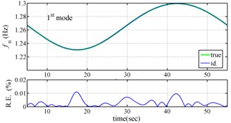
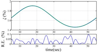
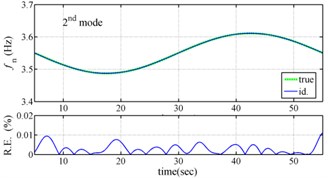
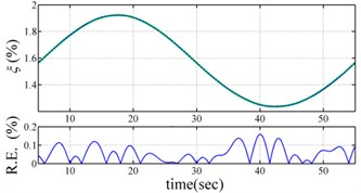
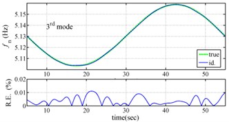
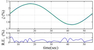
Fig. 3 present the comparison the identified instantaneous dynamic characteristics with true values for periodically varying system. The results of the proposed approach are highly accurate, with the relative errors of estimated frequencies much less than 0.02 % and the relative errors of estimated damping ratios much less than 0.3 %. The feasibility of the proposed approach is validated by the excellent agreement between the estimated instantaneous dynamic characteristics and true ones.

Fig. 1Numerical simulation model

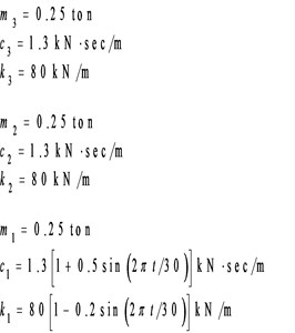
Fig. 2Simulated responses of a three-story time-varying shear building and the corresponding Fourier spectra

The spectrogram is a representation of visualization of the spectrum of frequencies or wave numbers in all kinds of process as they vary with time or space variable. The Gabor transform is a useful and popular method for getting the spectrogram of signal. Fig. 4 show the spectrogram of shear building subjected the Chi-chi earthquake. From these spectrograms the variation of each modal could be obtained, however, the resolution is too rough. Comparing the results obtained by the proposed approach with the Gabor-based spectrogram revealed that the present approach is substantially superior to spectrogram approach in estimating instantaneous dynamic characteristics. The success of the proposed approach, as revealed in capturing the variation of each mode, demonstrates the practical applicability of this procedure to a numerical model.

Fig. 3Comparison of estimated results with true values

4. Application to experimental responses

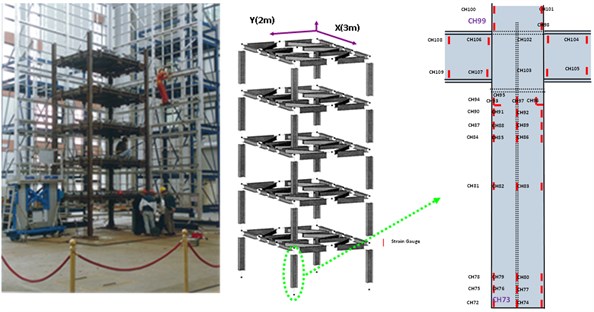
Shaking table tests are often carried out in a laboratory to examine the behaviors of structures in earthquakes. The Center for Research on Earthquake Eeegineering (NCREE) in Taiwan undertook a series of shaking table tests on a 3 m long, 2 m wide. And 6.5 m high steel frame to generate a set of earthquake response data of the five-story steel frame [23]. The mass of each floor with piled lead blocks was approximately 3664 kg. The displacement, velocity and acceleration response histories of each floor were measured with a sampling rate of 1000 Hz during the shaking table tests. Additionally, some strain gauges were installed in one of the columns and near the first floor (Fig. 5). Fig. 6 depicts the accleleration responses of all floors in the long-span direction, subjected to 60 % of the Kobe earthquake. The Fourier spectra of all floors that subjected to 8 % and 60 % of the Kobe earthquake are also given in Fig. 6.

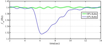
Yeh et al. Reported that the frame responded linearly when it subjected to 8 % of the strength of the Kobe earthquake, and the steel columns near the first floor yielded when the frame subjected to 60 % of the strength of the Kobe earthquake. Measured strains shown in Fig. 7 evidence the observations. The labeled “CH73” and “CH99” strain gauges be setted on the bottom of first and second floors, respectively (Fig. 5). There have been residual strains since t was around 6 seconds when the frame was subjected to 60 % of the Kobe earthquake. Because of the symmetry of the steel frame, only the acceleration responses and inputs in the long span direction were processed to find the instantaneous dynamic characteristics.

Fig. 4Spectrogram of three-story time-varying shear building subjected the Chi-chi earthquake

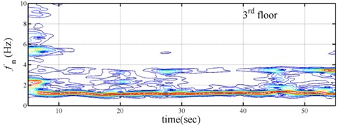
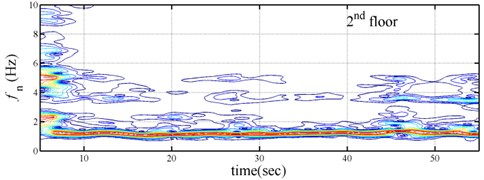
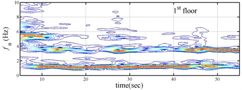
Fig. 5A photo, sketch and distribution of strain gauge of five-story frames

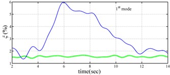
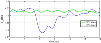
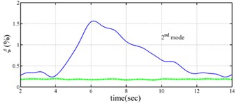
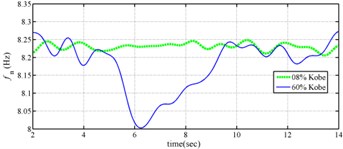
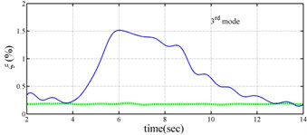
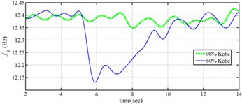
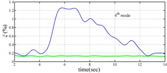
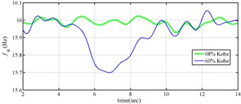
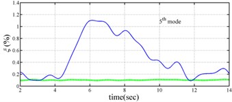
The measured acceleration responses of base and each floor relative to the base were used to apply the Gabor transform. The instantaneous dynamic characteristics show in Fig. 8 were estimated for the steel frame subjected to 8 % and 60 % of the Kobe earthquake. As expected, small variations of instantaneous natural frequencies with time are observed in Fig. 8 for the frame under 8 % of the Kobe earthquake because no damage occurred to the frame. The estimated instantaneous natural frequencies in the 8 % Kobe earthquake test are 1.39-1.41 Hz, 4.52-4.54 Hz, 8.20-8.25 Hz, 12.35-12.41 Hz and 15.95-16.05 Hz. The estimated instantaneous natural frequencies are close to the peak frequencies observed in the Fourier spectra (Fig. 6).

Comparison of the instantaneous dynamic characteristics estimated for 60 % Kobe input with those for 8 % Kobe input reveals that $f_{n} (t)$ estimated for 60 % Kobe input are generally smaller than those estimated for 8 % Kobe input. The estimated instantaneous natural frequencies in the 8 % Kobe earthquake test are 1.31-1.41 Hz, 4.35-4.55 Hz, 8.00-8.27 Hz, 12.10-12.41 Hz and 15.70-16.05 Hz. While $ξ (t)$ show the opposite trend. These observations obey the well-known physical phenomenon that damage in a structure induces the decrease of natural frequency and increase of damping ratio for the structure. Furthermore, significant decrease in $f_{n} (t)$ is observed at $t =$ 5.5 seconds around, especially for the first mode showing more than 6 % decrease in $f_{n} (t)$ , which indicates possible damage initiated in the frame at the moment. This finding with what is observed from the measured strains in Fig. 6.

Fig. 6Responses of five-story frame subjected 60 % Kobe earthquake and the corresponding Fourier spectra

Fig. 7Time history of strain gauge on the bottom of first and second floors

Fig. 8Instantaneous modal parameters obtained from experimental data

5. Conclusions

This work has presented a procedure for estimating the instantaneous dynamic characteristics of a time varying or nonlinear structure form its measured dynamic responses, using Gabor transform. To catch the time varying feature of the structure, the coefficient matrix of Auto-regressive time series model is assumed to be functions of time and calculated by weighted least square approach. The dynamic acceleration responses and input forces of the structural system are used to construct Auto-regressive time series model on Gabor frame. Then, the instantaneous dynamic characteristics of the structural system are directly estimated from the coefficient matrix of Auto-regressive time series model. The feasibility of the proposed procedure has been demonstrated by processing numerical simulated dynamic responses of a three-story shear building whose stiffness and damping at the first floor are time dependent.

To demonstrate the applicability of the present approach to real data, the present approach has also been applied to process the acceleration responses of a five-story steel frame, subjected to 8 % and 60 % of the Kobe earthquake, in shaking table tests. The frame was first shaken under 8 % Kobe input, then subjected to a 60 % Kobe input and yielded. The estimated instantaneous dynamic characteristics are consistent to the observed physical phenomena in the tests. The estimated instantaneous dynamic characteristics indeed indicate possible damage in the structure and when the damage initiated.

References

Wang Z. N., Fang T. A time domain method for identifying modal parameters. Transaction of ASME, Journal of Applied Mechanics, Vol. 53, Issue 1, 1986, p. 28-32.

Search CrossRef
Loh C. H., Wu T. S. Identification of Fei-Tsui arch dam from both ambient and seismic response data. Soil Dynamics and Earthquake Engineering, Vol. 15, Issue 7, 1996, p. 465-483.

Publisher
Huang C. S. Structural identification from ambient vibration measurement using the multivariate AR model. Journal of Sound and Vibration, Vol. 241, Issue 1, 2001, p. 337-359.

Search CrossRef
Lardies J. Modal parameter identification based on ARMAV and state-space approaches. Archive of Applied Mechanics, Vol. 80, Issue 1, 2010, p. 335-352.

Publisher
Su W. C., Huang C. S., Chen C. H., Liu C. Y., Huang H. C., Le Q. T. Identifying the modal parameters of a structure from ambient vibration data via the stationary wavelet packet. Computer-Aided Civil and Infrastructure Engineering, Vol. 29, Issue 10, 2014, p. 738-757.

Publisher
Huang C. S., Lin H. L. Modal identification of structures from ambient vibration, free vibration, and seismic response data via a subspace approach. Earthquake Engineering and Structural Dynamics, Vol. 30, Issue 12, 2001, p. 1857-1878.

Publisher
Ali M. R., Okabayashi T. System identification of highway bridges from ambient vibration using subspace stochastic realization theories. Earthquake and Structures, Vol. 2, Issue 2, 2011, p. 189-206.

Publisher
Ibrahim S. R., Mikulcik E. C. The experimental determination of vibration parameters from time responses. Shock and Vibration Bulletin, Vol. 46, Issue 5, 1976, p. 187-196.

Search CrossRef
Niedzwiecki M. Identification of Time-Varying Processes. John Wiley and Sons, New York, 2000.

Search CrossRef
Loh C. H., Lin C. Y., Huang C. C. Time domain identification of frames under earthquake loading. Journal of Engineering Mechanics, ASCE, Vol. 126, Issue 7, 2000, p. 187-196.

Publisher
Belge M., Miller E. I. A sliding window RLS-like adaptive algorithm for filtering alpha-stable noise. IEEE Signal Process Letter, Vol. 7, Issue 4, 2000, p. 86-89.

Publisher
Leung S. H., So C. F. Gradient-based variable forgetting factor RLS algorithm in time-varying environments. IEEE Transactions on Signal Processing, Vol. 53, Issue 8, 2005, p. 3141-3150.

Publisher
Marmarelis V. Z. Advanced Methods of Physiological System Modeling. University of Southern California, Los Angeles.

Search CrossRef
Zou R., Wang H., Chon K. H. A robust time-varying identification algorithm using basis functions. Annals of Biomedical Engineering, Vol. 31, Issue 7, 2003, p. 840-853.

Publisher
Huang C. S., Hung S. L., Su W. C. Identification of time-variant modal parameters using time-varying autoregressive with exogenous input and low-order polynomial function. Computer-Aided Civil and Infrastructure Engineering, Vol. 24, Issue 7, 2009, p. 470-491.

Publisher
Jiang X., Adeli H. Dynamic wavelet neural network for nonlinear identification of highrise buildings. Computer-Aided Civil and Infrastructure Engineering, Vol. 20, Issue 2, 2005, p. 316-330.

Publisher
Haggan V., Ozaki T. Modelling nonlinear random vibrations using an amplitude-dependent autoregressive time series model. Biometrika, Vol. 68, Issue 1, 1981, p. 189-196.

Publisher
Huang C. S., Hung S. L., Wen C. M., Tu T. T. A neural network approach for structural identification and diagnosis of a building from seismic response data. Earthquake Engineering and Structural Dynamics, Vol. 32, Issue 2, 2003, p. 173-185.

Publisher
Adeli H., Jiang X. Dynamic fuzzy wavelet neural network model for structural system identification. Journal of Structural Engineering, ASCE, Vol. 132, Issue 1, 2006, p. 102-111.

Publisher
Su W. C., Liu C. Y., Huang C. S. Identification of instantaneous modal parameters of time-varying system via a wavelet-based approach and its application. Computer-Aided Civil and Infrastructure Engineering, Vol. 29, Issue 4, 2014, p. 279-298.

Publisher
Wang Z. H., Fang T. A time-domain method for identifying modal parameters. Journal of Applied Mechanics, Vol. 53, Issue 1, 1986, p. 159-165.

Publisher
Huang C. S. Structural identification from ambient vibration measurement using the multivariate AR model. Journal of Sound and Vibration, Vol. 241, Issue 3, 2001, p. 337-359.

Publisher
Yeh S. C., Cheng C. P., Loh C. H. Shaking Table Tests on Scales Down Five-Storey Steel Structures. Report No. NCREE-99-002, Center for Research on Earthquake Engineering(NCREE), Taiwan, 1999.

Search CrossRef

About this article

Received

09 August 2016

Accepted

23 November 2016

Published

15 February 2017

SUBJECTS

Seismic engineering and applications

DOI

https://doi.org/10.21595/jve.2016.17894

Keywords

time varying

Gabor transform

instantaneous dynamic characteristics

Acknowledgements

The authors would like to thank the National Science Council of the Republic of China, Taiwan, for financially supporting this research under Contract No. MOST 105-2622-M-492-001-CC2. The appreciation is also extended to the National Center for Research on Earthquake Engineering for providing shaking table test data.

This is an open access article distributed under the Creative Commons Attribution License, which permits unrestricted use, distribution, and reproduction in any medium, provided the original work is properly cited.

Previous article in issue Previous Next article in issue Next

Research article

2023 11 27

Site effects based on time varying horizontal-to vertical spectral ratio

Fuchao Cao, Yinfeng Dong, Yiming Xie, Yiping Wang

Research article

2019 08 15

Tacholess order tracking method for gearbox based on time-varying filter and energy centrobaric correction method

Shuangxi Jing, Zhipeng Luo, Junfa Leng, Zhiyang Wang

Research article

2017 09 30

Moving window self-iteration PCE based OMA for slow linear time-varying structures

Tianshu Zhang, Cheng Wang, Jianying Wang, Yewang Chen, Yiwen Zhang

Research article

2017 03 31

Seismic performance of steel frames equipped with buckling-restrained braces (BRBs) using nonlinear static and dynamic analyses

Mahdi Eghbali, Esmaeil Asadian, Gholamreza Ghodrati Amiri, Seyed Ali Razavian Amrei

W.-C. Su and C.-S. Huang, “A study on Gabor frame for estimating instantaneous dynamic characteristics of structures,” Journal of Vibroengineering, Vol. 19, No. 1, pp. 447–457, Feb. 2017, https://doi.org/10.21595/jve.2016.17894

Copy Extrica

Copied to clipboard!

TY  - JOUR
DO  - 10.21595/jve.2016.17894
UR  - https://doi.org/10.21595/jve.2016.17894
TI  - A study on Gabor frame for estimating instantaneous dynamic characteristics of structures
T2  - Journal of Vibroengineering
AU  - Su, Wei-Chih
AU  - Huang, Chiung-Shiann
PY  - 2017
DA  - 2017/02/15
PB  - JVE International Ltd.
SP  - 447-457
IS  - 1
VL  - 19
SN  - 1392-8716
ER  - 

Copy Ris

Copied to clipboard!

@article{Su_2017,
	doi = {10.21595/jve.2016.17894},
	url = {https://doi.org/10.21595/jve.2016.17894},
	year = 2017,
	month = {feb},
	publisher = {{JVE} International Ltd.},
	volume = {19},
	number = {1},
	pages = {447--457},
	author = {Wei-Chih Su and Chiung-Shiann Huang},
	title = {A study on Gabor frame for estimating instantaneous dynamic characteristics of structures},
	journal = {Journal of Vibroengineering}
}

Copy Bibtex

Copied to clipboard!

[1]W.-C. Su and C.-S. Huang, “A study on Gabor frame for estimating instantaneous dynamic characteristics of structures,” Journal of Vibroengineering, vol. 19, no. 1, pp. 447–457, Feb. 2017, doi: 10.21595/jve.2016.17894.

Copy IEEE

Copied to clipboard!

Su, Wei-Chih, and Chiung-Shiann Huang. “A Study on Gabor Frame for Estimating Instantaneous Dynamic Characteristics of Structures.” Journal of Vibroengineering 19, no. 1 (February 15, 2017): 447–57. https://doi.org/10.21595/jve.2016.17894.

Copy Chicago

Copied to clipboard!

A study on Gabor frame for estimating instantaneous dynamic characteristics of structures

Abstract

1. Introduction

2. Theoretical formulation

2.1. Time-varying Auto-regressive time series model

2.2. Determination of instantaneous dynamic characteristics

3. Numerical verification

4. Application to experimental responses

5. Conclusions

References

About this article

Related Articles