Non-uniform embedding applications for synchronization analysis

1. Introduction

The synchronization phenomena have been intensively investigated due to its potential application in physical processes like communications [1, 2], system control [3], artificial analysis [4, 5], financial time series [6]; and biological processes, like neurophysiological systems [7] and cardiorespiratory rhythms [8]. Usually synchronization theory is based on phase synchronization [5, 9]. However, state space of the system can be reconstructed from their observations [10] and various geometrical and dynamic properties can be analyzed [11] and successfully applied in synchronization analysis [3, 12]. In past, a variety of the synchronization methodologies of chaotic vibration systems have been suggested, such as variable structure control approach, back stepping control approach and others [13, 14].

One of the main problems arising when designing of dynamical model is instability of a system [13, 15]. Assessing model based on its dynamic response requires synchronous response measurements. For modeling of dynamic synchronization the rules that governs the original system is required. To find those rules non-uniform embedding and polynomial approximation model have been invoked. Systems embedding is an important step in the process of modeling of a system [16]. Attractor embedding is used to characterize the dynamics of a true system represented by obtained vibration. The embedding theorem says that dynamical systems has the same topological properties and is better represented by delayed version of an observed vibration [17]. Embedding dimension and time delay are two parameters determining the reconstruction of a system by a delay coordinate method. There are several ways to determine embedding dimension like correlation dimension or neural networks [18, 19]. In this paper one of the classical methods called false nearest neighbor (FNN) method for identification of embedding dimension is used [20]. For identification of time delays computational techniques like mutual information or autocorrelation based methods often used [21]. However, in this paper we propose a simple way for time delay selection. For time delay identification, evolutionary optimization algorithms were introduced [16]. The problem of evolutional optimization is to identify optimal set of time delay that represents the best properties of reconstructed system. Polynomials approximation was used to construct the synchronization of vibrations [22]. Polynomials produce a good approximation to complex systems [23]. Polynomial model is derived using optimal non-uniform time delay coordinates.

For synchronization task we propose new iterative algorithm for polynomial construction. The synchronization was examined for vibration obtained by aquarium with air pump [24] and wind turbine pinion gear [25]. The model of synchronization is constructed in several steps. In Section 2 the signal reconstruction based on non-uniform embedding proposed in [16] was applied. Evolutionary optimization algorithms for identification of the optimal set of time delays are discussed in Section 3. In Section 4 synchronization model was defined. Simulation results for two vibrations are presented in Section 5. And concluding remarks are discussed in the final section.

2. Non-uniform embedding reconstruction of a signal

Let us consider discrete time series which is presented in form of $x_1$, $x_2$,…, $x_N$. The non-uniform reconstruction is obtained from original time series when the time delays between coordinates were chosen non-uniformly $Y_i=\left\{x_i,x_{i+{\tau }_1},x_{i+{\tau }_1+{\tau }_2},\dots ,x_{i+\sum _{k=1}^{d-1}{\tau }_k}\right\}$, $i=\mathrm{1,2},\dots ,N-\sum _{k=1}^{d-1}{\tau }_k$. The embedding dimension is denoted by $d$; $Y_i$ is the reconstructed vector with dimension $d$; ${\tau }_k\in N$ are the time delays.

First task of the reconstruction is to determine optimal embedding dimension. For this purpose the false nearest neighbors method was applied [20]. In this method, if two points become distant by increasing embedding dimension $d$ then one of them is supposed as false. Embedding dimension is chosen when there is no false nearest neighbours. The nearest neighbor in the $\left(d-1\right)$-th cycle is supposed as false if:

where $R_d^2\left(i\right)$ is the Euclidean distance of the $i$-th point in the $\left(d-1\right)$-th cycle to its nearest neighbour, $R_{d+1}^2\left(i\right)$ is the same distance in the $d$-th cycle with additional $x\left(t-{\tau }_d\right)$ time delay coordinate and $R_{tol}$ is a threshold [20].

The next step of time series embedding is to choose algorithm which helps to find the optimal set of time delays. This set gives best characteristics of the reconstructed attractor in $d$-dimensional space. For this case we use the objective function which was used for non-uniform attractor embedding in [16]:

where $Q\left({\tau }_1,{\tau }_2,\dots ,{\tau }_{d-1},\omega \right)$ is the embedding quality function Eq. (3) of reconstruction into time delay phase space. This quality function evaluates arithmetic average of all planar projection of reconstructed attractor [16]. Thus, if time series is reconstructed into $d$-dimensional time delay space there are $d\left(d-1\right)/2$ planar projection and quality function can be expressed as:

The maximum of the objective function Eq. (2) gives the optimal set of time delays {${\tau }_1,{\tau }_2,\dots ,{\tau }_{d-1}\}$. With this set of time delays chaotic attractor in the reconstructed space have optimal geometric properties.

3. Evolutionary algorithms for the identification of an optimal set of non-uniform time delays

As it was mentioned in previous section the non-uniform embedding can express the best topological properties of reconstructed signal [17]. Although this reconstruction is affective, but in this case an optimized set of all time delays ${\tau }_i$($i=$1, 2,…, $d-$1) must be identified. If the upper bound $T$ for possible numerical values of time delays are chosen, then the number of different combinations of time delays is the number of different combinations without permutations is $\left(T+d-2\right)!/(\left(d-1\right)!\left(T-1\right)!)$ [16]. For example, there is 292825 different combinations of time delays without permutations when $d=\text{5}$ and $T=$ 50. For higher dimension, it is infeasible to use full sorting. To solve this problem evolutionary optimization algorithms where used for identification for time delays. In this paper we use three different optimization algorithms which were adapted for identification of optimal set of non-uniform time delays.

4. Polynomial synchronization

Time series reconstruction into time delay space allows obtaining certain properties of attractor that can be used in system control. In most of these tasks synchronization of the system is needed. In this paper the synchronization problem is considered as a construction of a model for some dynamical system. Lets $g$ denote the dynamics of the time series:

where $X_{1i}=x_i$, $X_{2i}=x_{i+{\tau }_1}$,…, $X_{di}=x_{i+\sum _{k=1}^{d-1}{\tau }_k}$ is the time delayed vectors with dimension $d$ and set of time delays {${\tau }_1,{\tau }_2,\dots ,{\tau }_{d-1}\}$. However, the rule $g\left(\bullet \right)$ is unknown. In construction of synchronization model the principal rule is to find approximate function g which would be as close as possible to original dynamics $x$ (note that $x_{N+1},x_{N+2},\dots$ are known). Aim is to minimize the difference:

For construction of rule $g$ polynomials that provide good approximation to $x$ with proper structure selection were used [12, 22]. The number of terms in the polynomial expansion of $g$ grows with degree $n$ of the polynomial. There is $M=\sum _{i=1}^n\frac{\left(i+d-1\right)!}{\left(i\right)!\left(d-1\right)!}+1$ terms for polynomial of degree $n$ with $d$ variables. For example, there is $10$ terms for polynomial of degree $n=\text{2}$ and reconstruction dimension of $d=\text{3}$.

We consider the $n$-th order polynomial:

where ${\omega }_0$, ${\omega }_1$,…, ${\omega }_M$ is the coefficients of the polynomial and $X_{ki}$ ($k=$ 1, 2,…, $d$) time delay coordinates. The task is to find such ${\omega }_0$, ${\omega }_1$,…, ${\omega }_M$ values that the overall solution minimizes error $E$ described by Eq. (9). Polynomial regression model using linear least square techniques based on orthogonal triangular factorization with column pivoting was applied [32]. However, with high embedding dimension and high polynomial order the terms of polynomial also increases. In order to decrease the number of polynomial terms the new iterative reconstruction algorithm was applied.

The iterative polynomial approximation algorithm consist of two steps:

1-step. The second order polynomial $P_2\left(X_{1i},X_{2i},\dots ,X_{di}\right)$ is constructed and coefficient ${\omega }_0$, ${\omega }_1$,…, ${\omega }_M$ are optimized.

2-step. Increase the order of the predefined polynomial, by using Eq. (10) with additional variable, which is the second order polynomial constructed in first step:

This step is repeated until the error $E$ does not improve. Finally, the synchronization model is the last polynomial that is found after the optimization process:

For even order polynomial construction first order polynomials should be used in first step. Thus, in the same synchronization problem we optimize two polynomials of odd and even orders one-at-a-time. The final solution is the lower order polynomial which gives the minimal errors.

5. Experiments

The proposed method for signal synchronization based on non-uniform embedding works well with different vibrations. We will test this technique for a few different vibrations and then make some generalizations.

First for both vibrations Savitzky-Golay Filter was used [33]. The key idea of Savitzky-Golay Filter is that the smoothed value $z_i$ in the point $x_i$ ($i=$1, 2,…, $N$) is obtained by taking an average of the neighboring data. More generally we can also fit a polynomial through a fixed number of points. Then the value of the polynomial at $x_i$ gives the smoothed value $z_i$.

Case 1. First vibration used for this technique is vibration of aquarium with air pump [24]. Length of a vibration is 51 s and sampling rate is 100 Hz. Every vibration can be efficiently transformed in electrical energy and employed to power electronic devices. In order to achieve this and make a better use of energy the dynamics of vibration must be known.

Fig. 1Objective function value compared to number of generation. The thick line shows objective function value for uniform embedding. Upper thin line – is the maximum value of F for each generation. Middle thin line – is the mean value of F for each generation. Lower thin line – is the minimum value of F for each generation

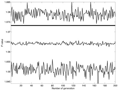
a) CS algorithm

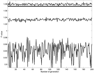
b) ABC algorithm

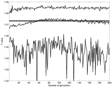
c) GA algorithm

First task of proposed model is to prepare the vibration for synchronization. For noise reduction Savitzky-Golay Filter was applied [33]. The second step was reconstruction into non-uniform time delay phase space. The False Nearest Neighbors algorithm suggested that embedding dimension is $d=\text{6}$. With next step the set of optimal time delays was identificated by evolutionary optimization algorithm. Refer to Fig. 1 for objective function value comparison to a number of generation for each optimization algorithm. The number of initial population for each algorithm was chosen equally. In each generation, all three-optimization algorithm were executed for 100 times. The thick line in Fig. 1 shows objective function value of uniform embedding. The thin lines show non-uniform embedding objective function value for each generation. As Fig. 1, shows each algorithm managed to find better objective function value than using uniform embedding.

The optimal set of time delays for uniform embedding is determined to be $F\left(\mathrm{9,9},\mathrm{9,9},9\right)=\text{1.0732}$. The non-uniform set of time delay is determined using evolutionary algorithms shown in Table 1. The set of time delay was chosen with the highest objection function value. This was obtained by Cuckoo Search algorithm. The optimal set for non-uniform embedding is determined to be $F\left(\mathrm{9,6},\mathrm{6,6},10\right)=$ 1.0851.

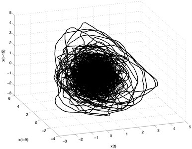
Refer to Fig. 2 for signal reconstruction into 3-dimensional time delay space using $X_1$, $X_2$, $X_3$.

Fig. 2Vibration reconstructed into 3-dimensional space with time delay set (X1,X2,X3) and using time delays τ1= 9 and τ2= 6

The 4-th order polynomial was build with found delays for this vibration. The found model have been given in Appendix A.1. The synchronization for real data and constructed polynomials is shown in Fig. 3. For polynomial approximation, we use 36 terms (while traditional model with polynomial order of 4 and reconstruction dimension $d=\text{6}$ would have 210 terms).

Case 2. Second vibration is radial vibration which measurements were taken on 3 MW wind turbine pinion gear. [25] Recorded length of a vibration is 6s and sampling rate is 97656 Hz. In this case we have high vibration levels. The same process was applied to this vibration as in Case 1. First Savitzky-Golay Filter was used to reduce noise of a signal. The False Nearest Neighbors algorithm suggested that embedding dimension is $d=\text{4}$. The non-uniform set of time delay is determined using evolutionary algorithms shown in Table 1. The best set of non-uniform embedding was found with Cuckoo Search algorithm $F\left(\mathrm{14,13,15}\right)=\text{1.1349}$. Refer to Fig. 4 for synchronization results. The 6-th order polynomial was build with found delays for this vibration. The found model have been given in Appendix A.2. The found model has a total 27 terms (while traditional model with polynomial order of 6 and reconstruction dimension $d=$ 4 would have 210 terms).

As expected synchronization performance was not high due to the complex nature of the vibrations (refer Fig. 4 for residual). Filtering reduces the complexity of vibration and improves synchronization results.

Fig. 3a) Synchronization of real vibration (solid line) and vibration obtained with polynomial model (dashed line), b) residual of obtained and real signal

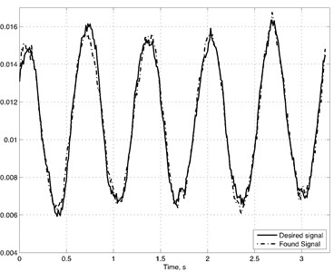
a)

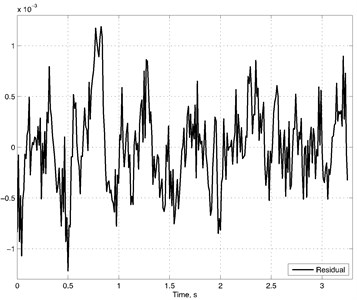
b)

Fig. 4a) Synchronization of real vibration (solid line) and vibration obtained with polynomial model (dashed line), b) residual of obtained and real signal

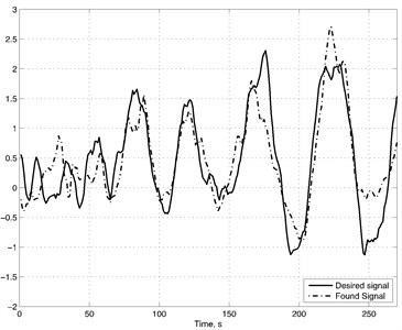
a)

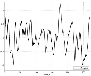
b)

6. Conclusions

It was demonstrated that synchronization of true dynamics and learnt model can be obtained by using polynomial model, which was derived using optimal non-uniform delay coordinates. This technique is based on combination of non-uniform embedding, evolutionary optimization algorithms and polynomial model. For identification of embedding dimension False Nearest Neighbor method was used, which is the easy and fast way to find minimal embedding dimension. For identification of set of non-uniform time delays three different evolutionary algorithms were used. The found set was used as a time delay kernel for polynomial construction. Synchronization was carried for two different real world vibrations. The proposed model showed good synchronization results.