Separation of motion techniques for trajectory optimization in flexible redundant robot manipulators

1. Introduction

The use of light arms is necessary when the weight and volume of manipulator are the main factor in reducing energy consumption. The most important advantages of flexible manipulator are appropriate maneuver and the adaptability to changing conditions of product [1, 2]. But control of end-effector due to vibration in these conditions is a major challenge that has involved many researchers by itself. The extra DOF or redundancy can play a role for freedom of action of manipulator in facing with obstacles, moving smoothly and avoid destructive accelerations, minimizing departure time and reducing vibration in flexible manipulators [3]. In these conditions, the tasks assigned to the robot can be obtained in different paths in the joint spaces and therefore, the optimal path is selected based on the goals of designers. Springer et al. [4] determined minimum time trajectory in conditions of avoiding resonance of elastic vibrations using generalized forces. Wilson et al. [5] obtained control torque by converting time optimal control problem to discrete dynamic programming. Choi et al. [6] used a method based on exact equilibrium manifolds in optimal trajectory planning. Bahrami et al. [7] developed optimal control of flexible space robots by using direct collocation method. They converted optimal control problem into standard nonlinear programming by using this technique and could achieve the minimum traveling time and actuating torque in point-to-point motion. Korayem et al. [8] used dynamic programming in determining the optimal trajectory of rigid manipulators in both motions along a specified path and point-to-point motion. They increase convergence speed using a method based on sequential quadratic programming. Wu et al. [9] proposed the optimal trajectory planning by using fourth-order curves to reduce the vibration of the flexible space robot. A number of evolutionary algorithms such as genetic algorithm, imperialist competition on optimal trajectory planning were used [10, 11]. In references [12, 13] developed indirect and sequential nonlinear programming methods in optimal path planning of flexible mobile manipulators. In references [14, 15] Pontryagin’s maximum principle was used for trajectory planning of flexible manipulators. Heidari et al. [14] investigated rest-to-rest motion of flexible manipulator. Almasi et al. [15] examined the movement of the mobile robot.

2. Method

Additional DOF allows the designers to consider the goals such as energy consumption or vibrations of robot tip and minimize them in addition to the assigned work to the robot. Most researchers consider the optimization of tracking error along with the vibrations of flexible components. On the other hand, the tip vibration hasn’t been separated of rigid motion. In this research, we are searching separation of elastic vibration of flexible components. This strategy looking for access to desired designing goals with considering of rigid motion of robot and minimizing the vibration as main preference. In suggested method, all possible answers will be obtained as rigid and redundancy conditions. Then, the trajectory which minimizes the global objective function will be resulted using open loop optimal control. The objective function and constraints of optimization problem will be selected based on conditions of point-to-point motion or the specified trajectory between. In each state, by suitably selecting the state and control signal, the objective function and constraints will be changed to standard form of an optimization problem. Primarily this method will be obtained for point-to-point motion and in continuing will be improved for movement on the specified path. Dynamic equations of the system are constraints of optimization problem in point-to-point motion. For condition of motion in the specified trajectory, kinematic equations are added to dynamic constraints. Dynamic equations will be made by computing kinetic energy and system’s potential and using Lagrange formulation and assumed mode method (AMM). Optimization could be employed to local and global optimization. Although global optimization has relatively complex calculations and more time consuming, but it is more efficient and accurate [16]. Global optimization is defined as an integral indicator during the entire path. As a result, a path among kinematic solutions will be selected that minimizes the special index. Global optimization will be used in this research. There are two direct and indirect methods for solving optimal control equations. In direct method, firstly control and state variables are discreted and the optimal control problem is converted to a nonlinear planning problem. Then, by considering auxiliary points in the specified path, time variable is removed from constraint equations [17]. Its advantage is that the differential equations are changed to algebraic equations and there is no need to solve boundary value problem [16]. These methods do not result in accurate answers and are often time consuming and aren’t efficient due to many parameters [5, 18]. Indirect methods change the optimization problem in to differential equations using optimality conditions and then solve them. In the direct methods are good selection when the DOF is high or different objectives are considered in optimization [19, 20]. Despite the computational complexities and the probability of non-convergence in indirect methods, these methods are relatively accurate and reliable. Hamilton-Jacobi-Bellman equation and Pontryagin’s maximum principle are two known methods in indirect methods which use calculus variation for conversion of optimization problem to a set of differential equations [8]. Because of the very high nonlinearities of system equations of flexible robot manipulator and too many parameters, a method based on Pontryagin’s maximum principle is used to solve the optimal control problem in this article. The first order differential equations are derived and ultimately lead to a TPBVP. Pontryagin’s maximum principle in comparison with other techniques doesn’t need to linearization of equations, differentiation of joint parameters and use of polynomials [12]. The rest of the paper is organized as follows. In Section 3, the dynamic equations of the manipulator will be introduced, while the formulation of optimization problem in point-to-point motion will be described in Section 4. In Section 5, we are going to explain the Pontryagin’s maximum principle. Section 6 is presented formulation of optimization for the specified trajectory. In Section 7, 3-link robot manipulator is simulated by two examples. Finally, we will summarize our results and make some conclusions.

3. Modeling of flexible manipulator

Fig. 1 shows manipulator which includes $N$ arms and its end arm is flexible. $M_i$, ${\tau }_i$and ${\theta }_i$ are the hub, torque of motors and relative angle of $i$th arm, respectively. In Fig. 1, $XOY$ is the inertial reference coordinate framework and $x_i{O}_i{y}_i$ is relative coordinate for each flexible arm which its center is the hub of $i$th link.

Fig. 1Flexible manipulator

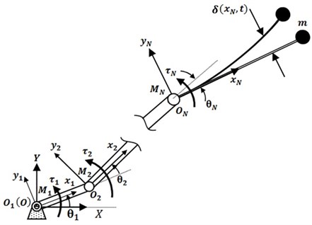
Flexible beam is considered as Euler- Bernoulli beam which means that the effect of shear deformation and rotational inertia is ignored. According to unlimited the dimensions of system in to flexible components, discretization method is commonly used for solving this problem. Assumed that the mode method is used to estimate the elastic deformation of flexible beam. In this method, deformation is considered by modal series in terms of mode shapes and time-varying variables [21]:

where $\delta$ is deformation, $x_N$, a general point on flexible beam, ${\psi }_j$ admissible functions, ${\varphi }_j$ time-dependent generalized coordinates and $M$ is number of modes. Reference [22] is represented calculating mode shapes and the natural frequencies. Kinetic energy of the manipulator is equal to the sum of kinetic energy of the arms, motors and load. We have:

where ${\mathbf{R}}_{M.i}$, ${\omega }_{M.i}$, $m_{M.i}$ and $I_{M.i}$ are position vector, angular velocity, mass and the moment of inertia of motors at joint $i$, respectively. ${\mathbf{R}}_i$ and ${\mathbf{R}}_m$ are the position vector on the $i$th arm and the payload to initial frame $XOY$ respectively. $m$ is load mass and${\rho }_i$, $A_i$ are the density and the cross section of the arms at joint $i$, respectively. Potential energy is resulted from elastic deformation and gravity. This energy is achieved as follows:

where $E_N$ and $I_N$ are Young modulus and the moment of inertia of flexible beam, respectively, and $g$, is gravitational acceleration. By substituting Eq. (1) in Eq. (3) the potential energy is calculated. The virtual work due to the torque ${\tau }_i$ would equal to ${\mathcal{W}}_i={\tau }_i\delta {\theta }_i$, therefore the equations of motion can be calculated using Lagrange method:

where $\mathcal{L}=T-P$ is Lagrangian and ${\theta }_i$ and ${\varphi }_j$ are the generalized coordinates. By calculating Lagrangian derivative with respect to the generalized coordinates and substituting in Eqs. (4) and (5), the equations of motion are extracted. By arranging the equations in matrix form, $n=N+m$ dynamic equations of motion will be as follows:

where $B$ is inertia symmetric matrix and consist of $B_{\theta \theta }\in {\mathfrak{R}}^{N\times N}$, $B_{\theta \varphi }\in {\mathfrak{R}}^{N\times M}$, $B_{\varphi \varphi }\in {\mathfrak{R}}^{M\times M}$. $D\in {\mathfrak{R}}^{n\times n}$ is damping matrix, $K\in {\mathfrak{R}}^{n\times n}$ is stiffness matrix and $\mathbf{F}\in {\mathfrak{R}}^n$ is sum of nonlinear force vectors such as coriolis, gravity and centrifugal. Also, ${\mathbf{h}}_{\theta }$ and ${\mathbf{h}}_{\varphi }$ are $M\times 1$ and $N\times 1$ vectors, respectively. $\ddot{\mathbf{\theta }},\dot{\mathbf{\theta }},\mathbf{\theta }\in {\mathfrak{R}}^{N\times 1}$ are angular position, velocity and acceleration vectors, respectively, and $\mathbf{\tau }\in {\mathfrak{R}}^{N\times 1}$ is torque vector of motors. The superscript $T$ in $B_{\theta W}^T$ denotes the transpose matrix.

4. Formulation of trajectory optimization in point-to-point motion

The motion of the manipulator is created point-to-point or moving in a pre-specified trajectory. This section, formulation of trajectory optimization in point-to-point motion is desired. Dynamic equations in Eq. (6) are system constraints in point-to-point motion. Because of the additional DOF in redundant flexible manipulator, a suitable indicator can be defined and minimized during the motion between two points. The method presented in this study is based on the separation elastic vibration of rigid motion. In fact, among the answers which exist for rigid motion of manipulator due to redundancy, we are looking for a response which minimizes vibrations of the system. In point-to-point motion, optimal trajectory of manipulators will be obtained by minimizing a value function comprehensively by considering dynamic constraints. So, the objective function is presented as follows:

where $t_s$ and $t_f$ are start time and end time of motion, respectively, and $\mathrm{\Omega }$, is function of designer goals. By rewriting the Eq. (6) dynamic constraints of system can be obtained as follows:

Also, unequal constraints are applied for bounding the torque and angular velocity magnitudes and to avoid saturation of operators and damaging to the system:

Unequal constrains can be acceded with consideration of the terms of torques and velocities in the objective function. To convert Eqs. (8) to (12) a standard form of an optimal control problem, the equations should be as follows:

where $\mathbf{u}$is the control signal vector. To convert to a standard form, $\mathbf{X}$ state vector is defined as follows:

Dimension of state vector $\mathbf{u}$ is considered as follows:

By using Eqs. (10) and (16), $\ddot{\mathbf{\varphi }}$ is obtained as follows:

$\dot{\mathbf{X}}$ is obtained by Eqs. (15), (16) and (17):

Also, vector $\mathbf{\tau }$ is obtained using Eqs. (9) and (17) as a function of $\mathbf{X}$, $\mathbf{u}$:

By substituting Eqs. (15) and (19) in (8) we have:

Consequently, Eqs. (8) to (12) are converted to standard form of the Eqs. (13) and (14).

5. Solution method and boundary conditions

Because of the large number of parameters in the equations of flexible manipulator, the indirect method is selected for optimal control problem. The main advantage of this method is its relatively accurate answers. Hamilton-Jacobi-Bellman equation and Pontryagin’s maximum principle are two known methods in indirect methods. The principles of two methods are based on the calculus of variations. In Pontryagin’s maximum principle, the optimization problem is converted to a series of first-order differential equations and boundary conditions for these equations are two points. This approach in comparison with other open loop optimal control techniques doesn’t have the need for equations linearization and differentiating with respect to joints parameters [23]. Pontryagin’s maximum principle states that if $u^{*}$ as optimal control is applied to a dynamic system of Eq. (6) and meets the conditions of optimal control Eqs. (13) and (14), must satisfy Hamilton equations in optimal points. According to this principle, we have:

where $\mathbf{\lambda }\in {\mathfrak{R}}^n$ is the vector of co-state variables. Hamiltonian, $\mathcal{H}$ is defined as follows:

One method to solve Eqs. (21) to (23) is the extraction of components of the vector $\mathbf{u}$ from Eq. (21) and substituting in Eqs. (22) and (23). By doing this, 2$n$ variables will be remained that need the same number of boundary conditions. In Pontryagin’s approach with the help of the calculus of variations, boundary conditions can be obtained as follows [24]:

Eq. (25) expresses boundary conditions in two initial $t_s$ and final $t_f$ points. Also, the position of end effector is specific in the first and last moment. Therefore, if $Z$ is the workspace dimensions of robot tip manipulator; we have 2$Z$ boundary conditions in two path terminals. Also, according to Eq. (25), in times of $t_s$ and $t_f$, vector $\mathbf{\lambda }$ is perpendicular to set of constraint equations. In other words, vector$\mathbf{\lambda }$ should be in raw space of Jacobean matrix. So, lying vector $\mathbf{\lambda }$ in column space ${\zeta }^T$ is equivalent to the presence of this vector in the null space of the matrix $I_N-{\zeta }^T{\left({\zeta }^T\right)}^{⋕}$ which can be written using linear algebra [25]:

Jacobean matrix $\zeta \in {\mathfrak{R}}^{Z\times N}$ of manipulator can be obtained as follows:

where $\mathbf{\sigma }$is the vector which specifies the location of end effector in terms of joint space of manipulator and ${\zeta }_{ij}$ is the arrays of Jacobean matrix. Eq. (26) has $n$-2$Z$ boundary conditions on each ends. Consequently, total of boundary conditions will be 2$n$ which is sufficient to solve the equations.

6. The formulation of optimization problem for moving in a specified path

To complete the discussion, some conditions are considered that the tip of manipulator moves between two points and in a specific path between them. In this case, the optimal space of joints will be changed by the presence of kinematic constraint. We consider the kinematic equation as follows:

In this relation, $\mathbf{\sigma }\left(\mathbf{\theta }\right)$ is a vector of tip position of manipulator and ${\mathbf{\sigma }}_d\left(t\right)$ is a vector of desired path and a function of time.

Eq. (28) is a nonlinear algebraic equation and there are countless answers for joint angles because of redundancy. By differentiation of the Eq. (28) we have:

where, Jacobin matrix $\zeta \left(\mathbf{\theta }\right)$ is obtained from Eq. (27). The null space $\zeta$ includes a variety of configurations of manipulator which result in a specific situation of the tip. Using this property, a state can be selected among different states which optimize a characteristic of the system. In this condition, the objective function of Eq. (8) and dynamic constraints of Eqs. (9) and (10) as well as kinematic constraint of Eq. (28) constitute the optimal control problem. To convert them into standard form equations, we differentiate by the Eq. (29):

$\mathbf{u}$ and $\mathbf{V}$ are defined as follows:

where $r\left(=n-Z\right)$ is the value of redundancy. Eq. (30) is rewritten with Eqs. (31) and (32):

So, angular acceleration vector $\mathbf{\theta }$ can be written as follows:

$\ddot{\mathbf{\varphi }}$, $\dot{\mathbf{X}}$, $\mathbf{\tau }$ and $g$ will be similarly obtained from Eqs. (17) to (20).

7. Simulation and results

In this section, the performance and the efficiency of the proposed method are studied by performing simulation and the results are discussed. As an example, we consider a 3-link robot with a third flexible arm. We assume that all the arms have a rectangular cross section and they move in a horizontal plane. Therefore, the workspace dimension is 2 ($Z=$ 2). The geometrical and mass properties are listed in Table 1. The arms are made of aluminum with the density and Young’s modulus of 2710 kg/m² and 71 GPa, respectively.

The mass, inertial moment and the gear ratio of the rotor are 0.2 kg, 0.02 kg.m² and 1, respectively. The payload mass is 250 gr. Two first natural frequencies are 6.27 and 91.23, respectively. In continuing, two examples would be considered for point-to-point motion and moving in specified path. In the first example, we evaluate the motion of the tip in point-to-point motion. The start and end point are (1.4, 0) and (1.27, 0.1), respectively. The DOF and redundancy are $N=$ 3 (regardless flexibility) and $r=$ 1, respectively. By considering two vibration modes, state and co-state vectors will be as follows:

Vector $\mathbf{u}$ is obtained according to redundancy and the Eq. (16):

We consider unequal constraint for the torque as follows:

where, we have ${\tau }_i^{+}=$ 0.06 N.m and ${\tau }_i^{-}=$ –0.06 N.m according to the relations Eq. (11). In applications, passing velocity from limit values causes damaging to the system. In these conditions, the joints velocity in the robot cannot exceed allowed values, and these velocities are bounded. Therefore, we consider the constraint for angular velocity as follows:

where, we have ${\dot{\theta }}_i^{+}=$ 0.06 rads and ${\dot{\theta }}_i^{-}=$ –0.06 rad/s according to relations Eq. (12) for limitation of joints velocity and torque of motors. According to the limitations of joints velocity and torque of motors, these factors are determined and should be considered in the objective function. The objective function is considered as a function of the squares of the joints velocity, elastic deformation of tip and energy consumption in the operators:

$w_{\varphi }$, $w_{{\tau }_i}$ and $w_{v_i}$, denotes penalty weights of elastic deformation, control signals and joints velocity respectively. Due to being the velocity and torque bounded, second and third terms are considered in Eq. (40). By substituting $w_v=w_{v_1}=w_{v_2}=w_{v_3}$ and $w_{\tau }=w_{{\tau }_1}=w_{{\tau }_2}=w_{{\tau }_3}$ into Eq. (40) and using Eqs. (19), (24) and (35) result to the Hamiltonian function as:

To study and appropriate conclusions, penalty factors are considered and compared in different situations. For this purpose, the following four cases are considered:

1. $w_{\varphi }\gg w_{\tau }$, $w_v$,

2. $w_{\tau }\gg w_{\varphi }$, $w_v$,

3. $w_v\gg w_{\tau }$, $w_{\varphi }$,

4. $w_{\tau }=1$, $w_{\varphi }=w_{\varphi }=50$.

By solving two-point boundary value problem, angles and optimal control command are obtained. The BVP4C command in MATLAB is used to solve first degree equation of systems with its boundary conditions. Also, uniform time networking with 100 points of $t_i\in \left[\mathrm{0,3}\right]$ where $i=$ 1,…, 100 have been used in simulation. Here we have $t_s=$ 0 and $t_f=$ 3 s. The initial guess for the first and second cases is 0.009 for angular positions, 0.7 for angular velocities and first and second five co-state variables are 0.0001 and 0.0002, respectively. The initial guess for the third and fourth cases is 0.2 for angular positions, first five co-state variables is 0.65, second five co-state variables 0.4 and remaining variables are zero. In this simulation to produce the optimal trajectory in addition to minimizing the objective function with respect to penalty matrices, joint velocities and torques shouldn’t exceed the limit values. Penalty matrices in cases 1 to 3 are considered to estimate limit conditions of these matrices. Case 4, according to the conditions of the problem is proposed as one of acceptable answers. The condition $w_{\varphi }\gg w_{\tau }$, $w_v$ ignores torque and velocity factors. Therefore, the only effective factor in the objective function is tip vibration. Torque and velocity are the only main factors for cases 2 and 3, respectively. Fig. 2 shows the trajectory of tip for cases 1 to 4. Fig. 2 shows that longer trajectory should be travelled to achieve the minimum vibration in the tip. In this case, the travelled trajectory is 33 cm which is twice the distance between two beginning and end points. Fig. 3 demonstrates the tip deflection for four cases. The maximum deformation for cases 1, 2 and 3 are 1.37, 4.31 and 4.91 mm, respectively, indicating that the tip vibration in the first case can reduce the maximum vibration up to three times in comparison with two other cases. In this condition, vibrating changes of tip between two initial and final peaks can be estimated by a line. Fig. 3 indicates this important point that peaks aren’t dependent on penalty matrices at the beginning and end of the path and occur at 0.09 and 2.88 seconds. Although the maximum vibration in cases 2 and 3 are close to each other, but vibration behavior is different in them. In the case 2 where $w_{\tau }$ is the determinant factor in the objective function, tip vibration is in oscillatory mode.

Fig. 2Tip trajectory

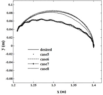
Fig. 3Tip vibration

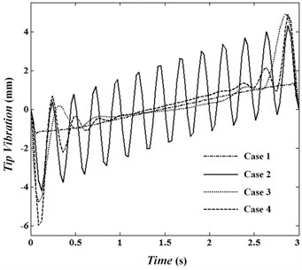
Fig. 4Angular velocity of joint 1

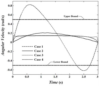
Fig. 5Angular velocity of joint 2

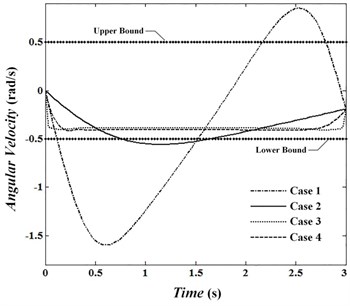
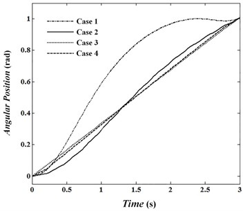
Angular velocities of joints are presented in Fig. 4 to 6 and Fig. 7 to 9 show the torque of motors for cases. In the first case, velocity in the joints reaches its maximum. The absolute value of velocities in this condition in the joints 1 to 3 are 0.82, 1.60 and 0.79 rad/sec, respectively and is passed by allowed value 0.5. In conditions $w_{\tau }\gg w_{\varphi }$, $w_v$, absolute value of angular velocity in second and third joints in its maximum value is 0.56 and 0.52, respectively which is passed limit value 0.5. By looking at Figs. 7 to 9 it can be concluded that changes of control torque in three joints can be estimated by a line. In this condition, the amount of energy consumption in operators has reached its lowest level. Fig. 10 shows angular velocities of joints for case 3. Fig. 10 shows that besides that the velocities are significantly reduced, the velocity changes are constant and has no significant change over time. In the third case, angular velocities in joint 1, 2 and 3 are reached constant values of 0.14, –0.39 and 0.34, respectively. Figs. 11 to 13 show produced angular positions for joints 1 to 3 for cases 1 to 4. Figs. 11 to 13 state that the changes of angular positions will be lined by increasing $w_v$. According to mentioned points and system responses in each case 1, 2 and 3, some conditions should be proposed to be of appropriate vibration in the tip meanwhile obtaining equal and unequal constraints of the problem. So, the fourth case in which $w_{\tau }=$ 1, $w_{\varphi }=w_{\varphi }=$ 50 is proposed. Penalty matrices are selected such that the behavior is close to the third case in velocity and second case in torque. Figs. 4 to 6 show that the angular velocities in the fourth case except at the beginning and end of the trajectory are close to the third case. For this condition, the maximum angular velocities (absolutely) are 0.15, 0.40 and 0.38 rad/sec for joint 1, 2 and 3, respectively. Also, Figs. 7 to 9 show that control torques except in path terminals are similar to the second case. The maximum absolute values of the torques in joints 1 to 3 are 0.055, 0.020 and 0.046 N.m, respectively, which has met the conditions of not crossing the limit value 0.06. Also, in this condition, tip vibration at the beginning and end of the movement is with trivial oscillation and approaches the line in the middle of the trajectory which is similar to behavior of cases 1 and 3. Anyway, meeting optimal conditions for all factors isn’t simultaneously possible and penalty matrices can be selected to achieve the intended result depending on their importance.

Fig. 6Angular velocity of joint 3

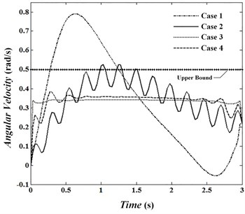
Fig. 7Torque of motor 1

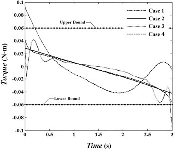
Fig. 8Torque of motor 2

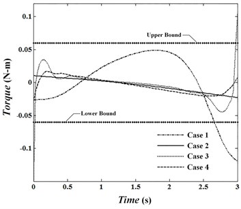
Fig. 9Torque of motor 3

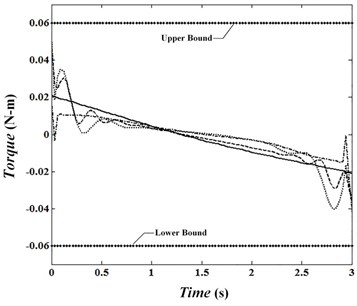
Fig. 10Angular velocity in case

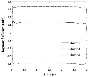
Fig. 11Angular position of joint 1

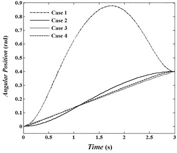
Fig. 12Angular position of joint 2

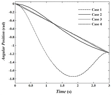
Fig. 13Angular position of joint 3

In the second example, the motion of the robot tip in the specified path is considered. Initial and end points are similar to the first example. The path of tip is considered as a circle with a radius of 0.1 and center (1.3, 0) in $XOY$ plane. Unequal constraints are considered to limit the torque and tip error as follows:

where $e$ is error of tip motion and ${\tau }_i^{+}=$ 0.06 N.m and ${\tau }_i^{-}=$ –0.06 N.m. The objective function is selected as follows:

$w_x$ and $w_y$ are the penalty weights for error of tip trajectory and $x_e$, $y_e$ are the coordinates of tip position in $x$ and $y$ directions, respectively. In this example, the angular velocities of motors are not considered as a determining factor. State and co-state vectors are relations Eqs. (35) and (36). Vector $\mathbf{u}$ is obtained by Eq. (31) as follows:

To study the effect of the penalty weights, we compare the following cases:

5. $w_e\gg w_{\varphi }$, $w_{\tau },\mathrm{}$

6. $w_{\varphi }\gg w_e$, $w_{\tau },\mathrm{}$

7. $w_{\tau }\gg w_e$, $w_{\varphi },$

8. $w_{\tau }=14$, $w_e=40$, $w_{\varphi }=1$.

Fig. 14 shows the tip trajectory in desired condition and for cases 5 to 8. Figs. 15 and 16 show tip trajectory error and tip vibration in four cases, respectively. Error of trajectory tracking in case 5 has the least error.

Fig. 14Tip trajectory

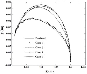
Fig. 15Error of tip trajectory

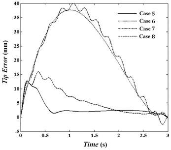
Fig. 16Tip vibration

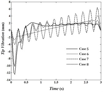
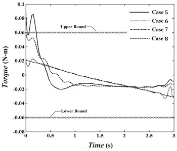
Fig. 17Torque of motor 1

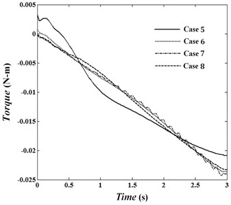
In this situation, the absolute value of the torque shouldn’t cross limit value 0.06 N.m. Figs. 17 to 19 show torques of motors in joints 1 to 3 for cases 5 to 8. In cases 6 and 7, penalty matrices of elastic bending and control commands are more in comparison with the remaining penalty matrices. Therefore, in case 6 the least deformation and in case 7 the least torque is seen. The maximum trajectory error is 12.7 mm in case 5 less than the bound of 16 mm. While Fig. 19 indicates that the maximum torque in this case is 0.088 N.m and is exceeded bound ${\tau }_i^{+}$. Penalty matrices are selected in case 8 such that while not crossing control commands of limit value and the error does not exceed 16 mm. The objective function is obtained 1.29 for this condition. Fig. 16 shows that by increasing $w_{\varphi }$ towards penalty matrices of error and torque, deformation can be estimated by a line. Minimum and maximum vibration of tip for case 6 are –2.7 mm and 4.1 mm and its average absolute value is 1.44 mm. What ever $w_{\varphi }$ decreased and $w_{\tau }$ increases, the range of vibration reaches to 2.85 mm in the middle of movement. Fig. 16 shows the first overshoot is at 0.12 second for each of four cases. In these circumstances, the maximum elastic deformation is occurred in fifth case and its value is –12.46 mm. By increasing $w_{\tau }$, in comparison with penalty matrices of error and deformation, the torques approach straight line. Also, in positions 6 and 7 in which penalty matrices of $w_{\tau }$ and $w_{\varphi }$ are more in comparison with remaining penalty matrices, the torques are close to each other and a trivial difference is seen between them. Obtaining optimal conditions depends on selecting penalty matrices and will be determined according to the intended conditions and objectives.

Fig. 18Torque of motor 2

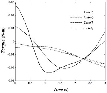
Fig. 19Torque of motor 3

Important conclusions are briefly summarized as follows:

The first and last overshoot in elastic deformation not depended on penalty matrices. When the penalty matrices of deformation, error (when moving in the specified path), torque and velocity are located as main priority in their maximum value compared to the rest of penalty matrices, the changes of these parameters can be estimated in linear form. Using unequal constraints, torque, velocity or error limitations are applied to the system. In these circumstances, in the event of selecting penalty matrices improperly, there is the possibility of damage to the system (for example, operators’ saturation). Obtaining optimal conditions aren’t possible for all indicators simultaneously and depending on the priorities considered, they can be adjusted to the desired result. For this work to predict the response of the system (relative to the penalty matrices), boundary conditions of these matrices considered similar to the conditions in cases 1 to 4 (or 5 to 8) can be investigated.

8. Conclusions

In this paper, designing trajectory optimization of flexible manipulators with redundancy in point-to-point motion and moving in a specified path was presented. This research suggests new optimal control based on the separation of vibration motion in flexible components. The goal of this strategy is access to the desired objectives of design by considering rigid motion of the robot and minimizing the vibration as the main priority. In the proposed method, all possible solutions are obtained based on rigid conditions and redundancy of the manipulator. Then, the trajectory which minimizes the global objective function was obtained using the open loop optimal control. In this research, according to nonlinear model of manipulator which is under equal and unequal non constraints, open loop optimal control method has been used. The goals depending on the conditions of point-to-point motion or movement on a specific trajectory between two points are different. In both conditions, maximum decrease of elastic vibrations of flexible members is considered as one of the main objectives. In each one by selecting state vector of the system and control signal properly, the objective function and constraints are converted to a standard optimization problem. The constraint in point-to-point motion includes differential equations in the system and unequal constraints. Objective function in these conditions includes terms of energy consumption in operators, joint velocities and elastic deformation. In the conditions of moving in a specified path, kinematic constraint is added to the constraints. In addition to the above constraints, unequal constraints are added to the problem to limit the torque and velocity in the joints. Due to the unlimited dimensions in flexible components, AMM was used for discretization and estimate of elastic deformation. Then by calculating kinetic and potential energy of the system and using Lagrange formulation, equations of motion were derived. To verify mathematical modeling and presented optimization method, simulation of three-link flexible manipulator was presented in two examples. The first example was conducted for point-to-point motion and the second one for moving in a specified path between two fixed points. In these circumstances, an additional DOF was used to minimize the objective function. Based on the desired objectives and unequal constraints for each example, objective function was defined associated with them. In point-to-point motion, objective function, including terms of elastic deformation of tip, energy consumption in operators and joint velocities were considered and trajectory error was replaced by velocities in moving in a specified path. System responses were analyzed in different conditions of penalty matrices. The results showed that there is no a unique solution that can satisfy all the goals. Therefore, appropriate trajectory can be selected to meet the desired goals by adjusting penalty matrices properly. Investigating the response of the system in different conditions and obtained results indicate the appropriate efficiency and accuracy in the proposed method.